Synopsis

Electrical properties imaging relies on accurate transceive phase determination. We explored the use of PLANET, an ellipse fitting approach on phase-cycled bSSFP data, for transceive phase mapping for the first time. We compared its accuracy, precision and time-efficiency with conventional SE and bSSFP techniques. Additionally, we reconstructed conductivity maps based on these techniques. We found that bSSFP and PLANET were as accurate as SE, but more precise. Also, bSSFP was the most time-efficient. Nevertheless, banding artefacts corrupting bSSFP transceive phase were, instead, intrinsically removed by PLANET. PLANET had clinically acceptable scan-time and was generally more suitable for conductivity mapping.

Introduction

Electrical Properties Tomography¹ requires mapping of the transceive phase $$$\phi^{\pm}$$$, which consists of RF transmit ($$$B_1^+$$$) and receive field ($$$B_1^-$$$) contributions. This transceive phase is commonly measured with the Spin-Echo (SE)². Alternatively to long SE acquisitions, bSSFP was introduced³ because of its high SNR and time efficiency. Nevertheless, bSSFP is prone to banding artefacts which compromise the phase pattern.

Phase-cycled (PC)-bSSFP has been shown to remove such bandings^4,5. Based on PC-bSSFP, a new methodology called PLANET⁶, introduced for $$$T_1$$$ and $$$T_2$$$ mapping, allows reconstruction of banding-free images and, additionally, maps off-resonance ($$$\Delta B_0$$$) and transceive phases.

Here, we investigate the accuracy, precision and time-efficiency of PLANET for transceive phase mapping for the first time, and we compare it with aforementioned techniques. Additionally, we compare conductivity, $$$\sigma$$$, maps reconstructed with standard MR-EPT using the transceive maps measured with these techniques.

Methods

MR measurements (3T, Philips Ingenia, Netherlands) were performed on a two-compartment, agar-based, cylindrical phantom and on the brain of a healthy volunteer with the body coil for transmission, and a 15-channel head coil for reception. A vendor specific algorithm (CLEAR) was used to remove the head coil receive sensitivity⁷. This resulted in phase images where only transmit and receive field contributions of the body coil were imprinted.

Table 1 summarizes phantom characteristics and imaging parameters used for SE, PLANET and bSSFP (corresponding to the 1^st phase cycle of PLANET). Each technique was run with five different resolutions. MR measurements were repeated with opposed gradient polarity to compensate for eddy currents.

To assess the precision of the measured transceive phase, a 2D parabola was fitted on the inner compartment. Given the homogeneous conductivity of this compartment, a 2D parabola is the expected shape of the transceive phase⁸. Deviations, as measured by the RMSE, were attributed to transceive phase uncertainty $$$\Delta \phi^{\pm}$$$. This uncertainty was then multiplied by the measurement time to derive the sequence efficiency.

Finally, the transceive phase assumption¹, and phase-only EPT⁹ were used for conductivity reconstructions. For both phantom and human brain, a 2D, noise-robust, derivative kernel (7x7 voxels)^9,10 was used for Laplacian computation.

Results & Discussion

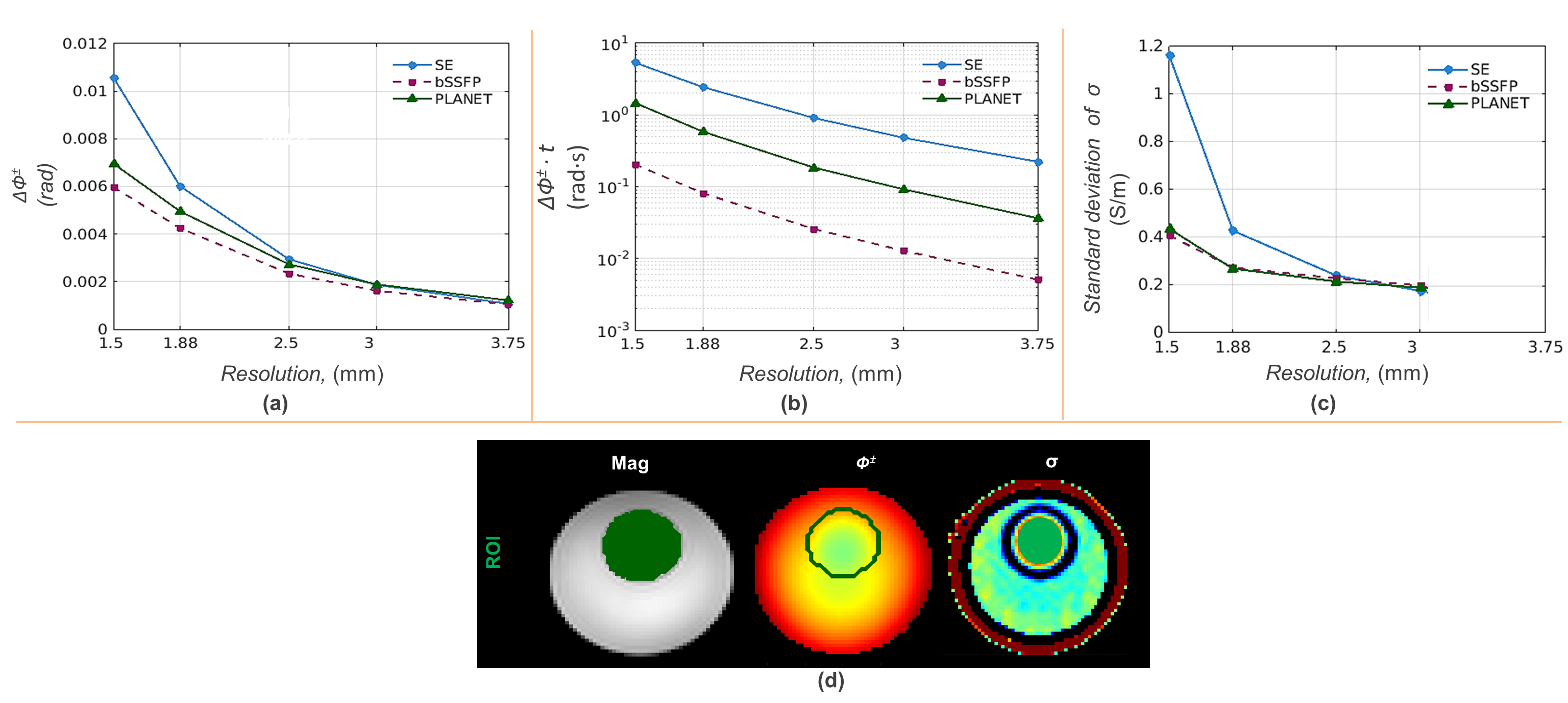
In Figure 1, the precision and efficiency of the three sequences were evaluated. Despite the lower SNR of SE (Fig. 2), $$$\Delta \phi^{\pm}$$$ was similar for the three techniques at resolutions $$$\geq$$$ 2.5 mm³ (Fig. 1a). For smaller voxels, $$$\Delta \phi^{\pm}$$$ was lower for bSSFP than PLANET and SE. After correction for scan-time (Fig. 1b), bSSFP out-performed PLANET and SE at all resolutions (factor 8 for PLANET, for SE a factor 20-34 at 1.5-3.75 mm³, respectively).

These results showed that addition of (phase-cycled) dynamics, as required by PLANET, did not result in the SNR improvement with respect to bSSFP, as one would naively expect ($$$\sqrt{8}$$$, based on 8 subsequent bSSFP images used for this technique). This may be attributed to various factors. First, the average SNR over the phase cycles in PLANET is lower than the SNR for bSSFP (Fig. 2), as PLANET uses modulation in signal amplitude for fitting purposes. Second, the fitting of additional parameters ($$$T_1$$$, $$$T_2$$$, banding free image, $$$\Delta B_0$$$) apparently leads to additional error propagation. Nevertheless, PLANET automatically corrected for off-resonance-induced bands (Fig. 2) and was more time-efficient than SE.

In Figure 1c, the conductivity standard deviation (SD) values are shown for the three transceive phase mapping methods. The SD of conductivity in the same ROI used for $$$\Delta \phi^{\pm}$$$ estimation generally confirmed transceive phase precision trends.

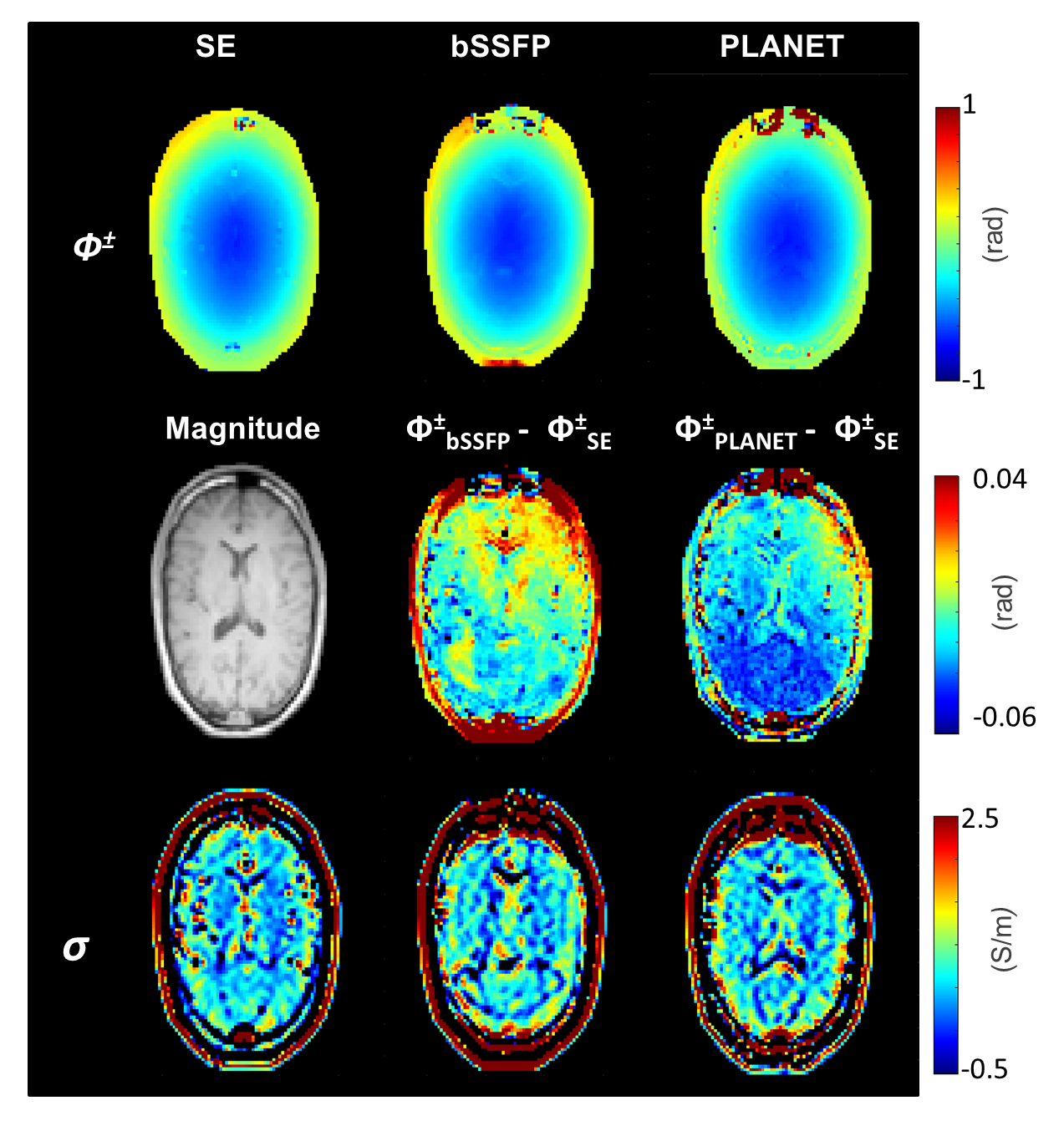
Figure 3 depicts the results obtained in the brain at 2.5 mm³ resolution. The transceive phase difference error for bSSFP and PLANET with respect to SE were comparable (less than 10%). This led to comparable conductivity maps. However, to ensure a steady-state regime for tissues with long relaxation times (e.g. CSF), extra dummy pulses were required. This resulted in extra scan time of 10 s per phase cycle, leading to a longer acquisition for both bSSFP and PLANET. Still, PLANET was 2.5 minutes faster than SE.

Conclusions

Acknowledgements

References

1. Katscher U & van den Berg CAT. Electric properties tomography: Biochemical, physical and technical background, evaluation and clinical applications. NMR Biomed. 2017;30:e3729.

2. Katscher U et al. Determination of electric conductivity and local SAR via B₁ mapping. IEEE Trans Med Imaging. 2009;28(9):1365–74.

3. Stehning C et al. Electric Properties Tomography (EPT) of the Liver in a Single Breathhold Using SSFP. Proc 20th Sci Meet Int Soc Magn Reson Med. 2012;386.

4. Bangerter NK et al. Analysis of Multiple-Acquisition SSFP. Magn Reson Med. 2004;51(5):1038–47.

5. Xiang QS & Hoff MN. Banding artifact removal for bSSFP imaging with an elliptical signal model. Magn Reson Med. 2014;71(3):927–33.

6. Shcherbakova Y et al. PLANET: An Ellipse Fitting Approach for Simultaneous T₁ and T₂ Mapping Using Phase-Cycled Balanced. Magn Reson Med. 2017;0:1–12.

7. Voigt T et al. Patient-individual local SAR determination: In vivo measurements and numerical validation. Magn Reson Med. 2012;68(4):1117–26.

8. Katscher U et al. Estimation of breast tumor conductivity using parabolic phase fitting. Proc 20th Sci Meet Int Soc Magn Reson Med. 2012;3482.

9. van Lier ALHMW et al. B₁⁺ Phase mapping at 7T and its application for in vivo electrical conductivity mapping. Magn Reson Med. 2012;67(2):552–61.

10. Mandija S et al. Error Analysis of Helmholtz-based MR-Electrical Properties Tomography. Magn. Reson. Med. 2017; early view. doi: 10.1002/mrm.27004.

11. Stogryn A. Equations for Calculating the Dielectric Constant of Saline Water. IEEE Trans Microw Theory Tech. 1971;19(8):733–6.

12. Kellman P & McVeigh ER. Image reconstruction in SNR units: A general method for SNR measurement. Magn Reson Med. 2005;54(6):1439–47.

13. Björk M et al. Parameter estimation approach to banding artifact reduction in balanced steady-state free precession. Magn Reson Med. 2014;72(3):880–92.