5081

Electro-Magnetic Property Mapping Using Kalman Filtering with a Single Acquistion at 3.0 T and 7.0 T MRI
Han-Jae Chung1,2, Jong-Min Kim1,2, You-Jin Jeong1,2, Jeong-Hee Kim3, Chulhyun Lee4, and Chang-Hyun Oh1,2

1Electronics and Information Engineering, Korea University, Seoul, Republic of Korea, 2ICT Convergence Technology for Health and Safety, Korea University, Sejong, Republic of Korea, 3Research Institute for Advanced Industrial Technology, Korea University, Sejong, Republic of Korea, 4Korea Basic Science Institute, Cheongju, Chungbuk, Republic of Korea

Synopsis

The phase-based Electro-Magnetic (EM) MR property imaging such as Quantitative Susceptibility Mapping (QSM) and MR Electric Properties Tomography (MREPT) shows great potential clinically. The main post-processing steps in QSM and MREPT are high-pass filtering and Laplacian of MR images. They, however, cause severe artifacts and noise during conventional calculations. In this work, we propose a novel reconstruction method of EM property MRI using Kalman filter algorithm and show the utility of the proposed method by comparing the imaging results.

Introduction

Recently, Electro-magnetic (EM) property imaging from Magnetic Resonance (MR) phase data such as Quantitative Susceptibility Mapping (QSM) and Magnetic Resonance Electric Properties Tomography (MREPT) have been studied to provide cross-sectional images of conductivity, permittivity, and susceptibility distributions inside the human1,2. However, these methods prone to cause serious artifacts in the conventional computation of High-Pass Filter (HPF) and Laplacian, the major post-processing steps of QSM and MREPT. In general, the HPF for background bias removal is usually performed by subtracting the low-pass filtered (LPF) data in spatial or frequency domain ($$$\phi_{HPF}=\phi-LPF(\phi)$$$), which causes the low frequency distortion. And, in the phase based MREPT ($$$\sigma=\frac{\triangledown^2\phi_{0}}{2\omega\mu}$$$), the Laplacian operator enhances the high-frequency noise and data loss near the edge between the tissues, resulting in unreliable mapping. In this study, we propose a new reconstruction method using Kalman filter algorithm to operate HPF and Laplacian as the 1st and 2nd order differential in the spatial domain directly and to reduce noise and artifacts in the resulting EM property images.

Methods

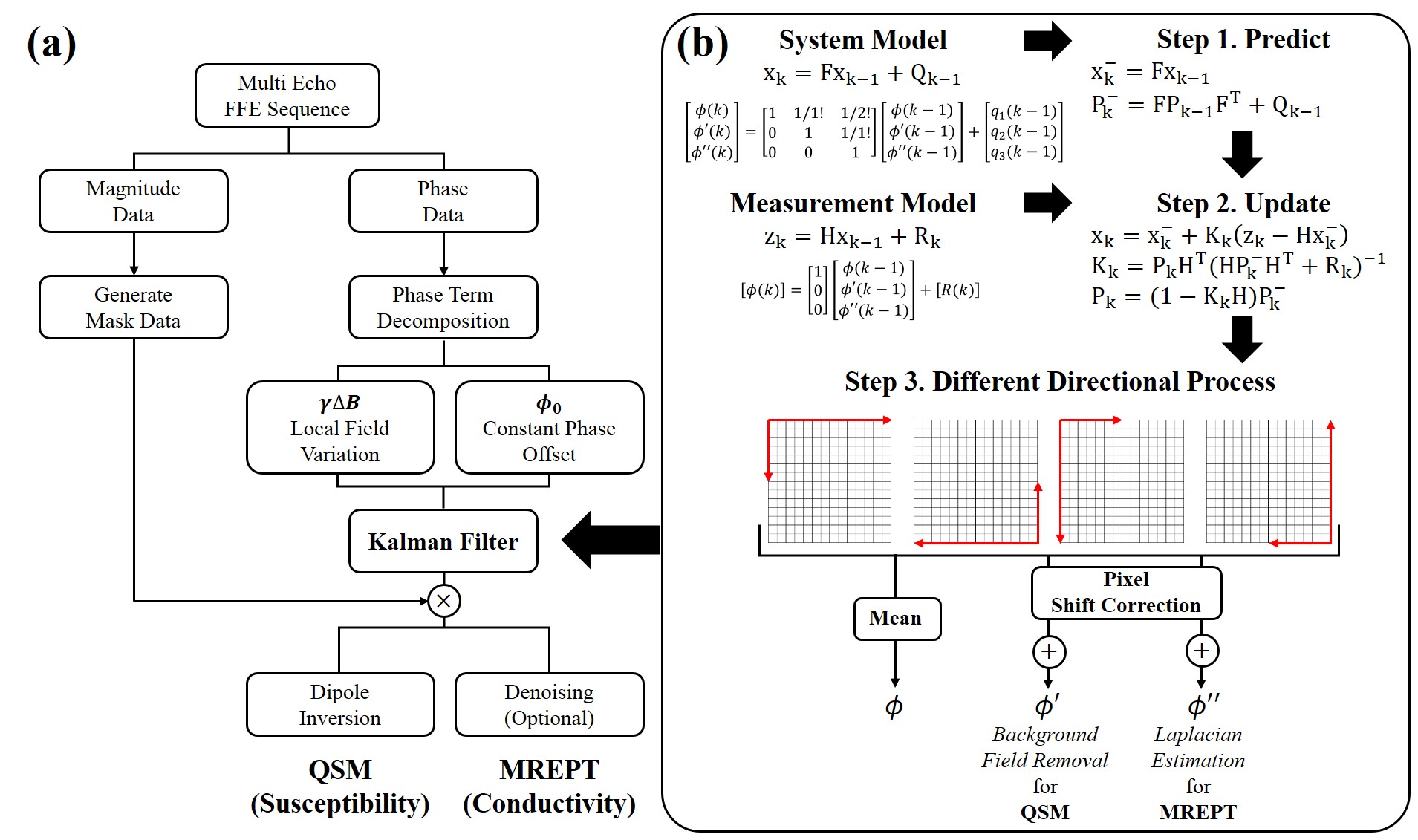
1. Kalman Filter Algorithm

To apply Kalman filter in the MR phase image, the measured phase is transformed to Taylor series form, $$$ϕ=ϕ+\frac{1}{1!} ϕ'+\frac{1}{2!} ϕ''$$$, under the assumption that it is sufficiently smooth. This can be modelled in a matrix form as in Fig. 1b. According to the system model, it is possible to estimate the images up to the second-order differential by using only measured phase image through the update and prediction process.

To maximize the performance, the Kalman filter is applied in four different directions, which improves the SNR resulting in better estimation of differential images (Fig. 1b). Finally, we obtain the 1st and 2nd order differentials which can be used for HPF in QSM and Laplacian in MREPT, respectively.

2. Data Acquisition

In-vivo experiments were performed on a 3.0 T and 7.0 T Achieva MRI Systems (Philips, The Netherlands). Data sets were scanned using multiple Fast Field Echo sequence and scan parameters were as follows: TR/TE1/$$$\triangle$$$TE (ms) = 530/4.1/3.8 on 3.0 T MRI, 1345/2.6/2.3 on 7.0 T MRI, FA = 18°, spatial resolution = 1×1×5 mm3, FOV = 256×256 mm2, number of signal measurements = 3, and number of echoes = 5.

For validation of MREPT, the Finite-Difference-Time-Domain (FDTD) simulations were conducted using Sim4Life (ZMT AG, Zurich, CH) and Duke human model with a 12-leg birdcage coil at 127.74 MHz.

Results

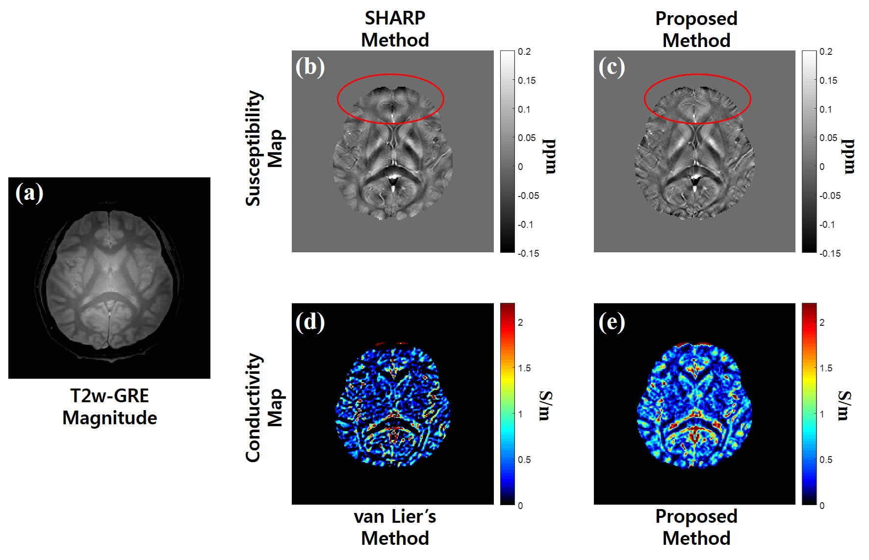
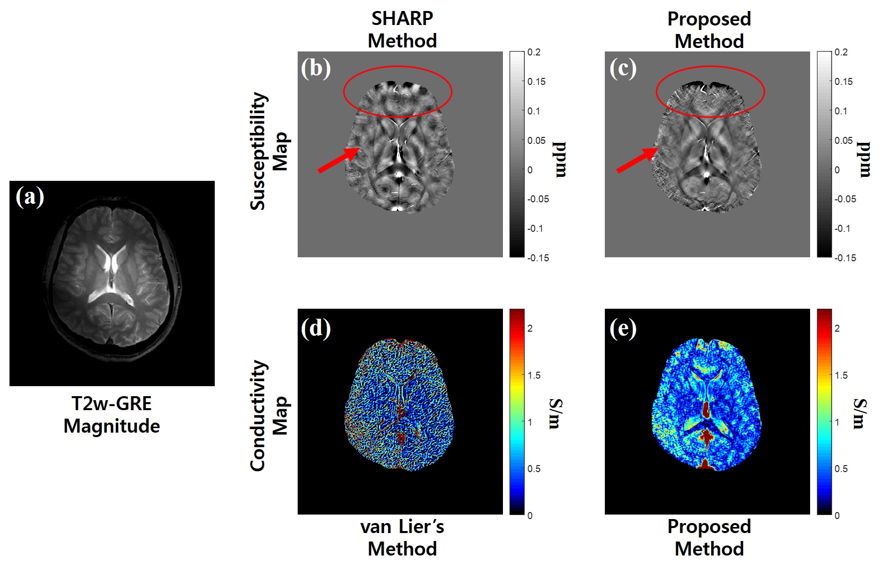
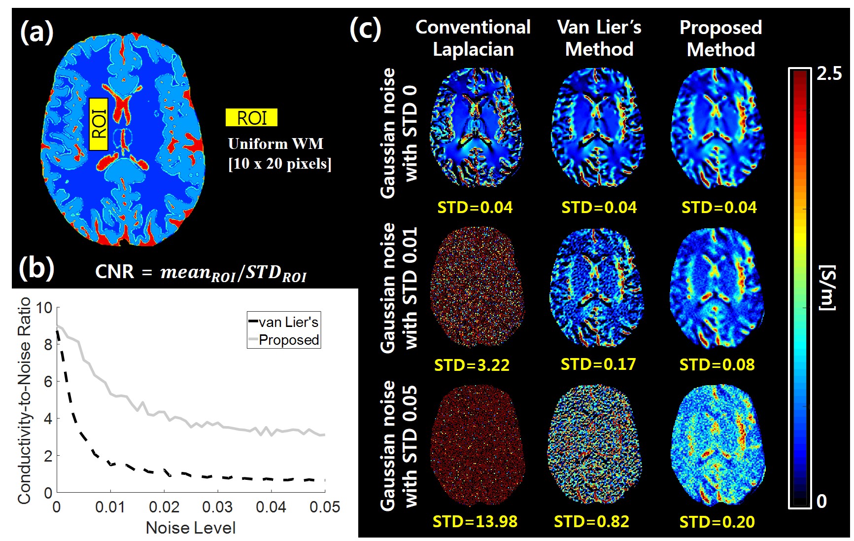
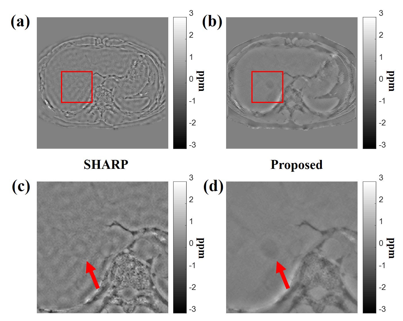
Figures 2 and 3 show the magnitude image and corresponding EM property maps computed by conventional and proposed methods at 3.0 T and 7.0 T, respectively. The mean of conductivity values are as follows: $$$\sigma_{Kalman}$$$(WM/GM/CSF) = 0.33/0.73/ 2.04 at 3.0 T, 0.31/0.77/1.31 at 7.0 T. Figure 4 shows the conductivity map reconstructed from the FDTD simulation with different noise levels whose standard deviation (STD) is 0 to 0.05. Figures 4b and c shows the conductivity-to-noise ratio and computed conductivity map when Gaussian noises of STDs of 0, 0.01, and 0.05 are added. Here the ROI was set in a uniform white matter region of 200 pixels (Fig. 4a). Figure 5 shows the abdomen QSM images obtained at 3.0 T for the whole body mask (and zoomed images) where the clear image is obtained for the proposed method compared with the conventional one.

Discussion & Conclusions

For QSM, SHARP3 was used as conventional background bias removal and dipole inversion was simply done by threshold based k-space division4. For MREPT, van Lier’s noise-robust kernel5 was used as a conventional Laplacian operator for performance comparison. The results show clear superiority of the proposed method over the conventional one. SHARP has low frequency distortion caused by imperfect background bias removal and higher magnetic field intensity. However, by using the proposed method, artifacts were reduced substantially in both 3.0 T and 7.0 T MRI as shown in red circles and arrows in Figs. 2 and 3. The definite difference between two methods can be seen in case of abdomen QSM (Fig. 5). In MREPT, without any denoising methods, our proposed method improved SNR by at least twice resulting in better contrast in experiments and simulations, also shown as Figs. 4b and c. However, due to reciprocity-theorem-based transceiver phase assumption does not work well in ultra-high field MRI system, there are some other challenges on 7.0 T conductivity imaging. In conclusion, we have proposed a novel spatially dependent filtering via Kalman filter algorithm in MR phase map and verified the utility of the proposed EM property mapping method. Background artifacts in QSM were substantially reduced by our Kalman filter based HPF in spatial domain without any subtraction of LPF data which makes frequency distortion in susceptibility map and pre-pixel dependent recursive tracking via four different directional Kalman filtering worked well.

Acknowledgements

This research was supported by the Next-generation Medical Device Development Program for Newly-Created Market of the National Research Foundation (NRF) funded by the Korean government, MSIP(NRF-2015M3D5A1065997).

References

1. Reichenbach JR, et al., Quantitative susceptibility mapping: concepts and applications. Clin Neuroradiol. 2015; 25: 225-230.

2. Katscher U, et al., Recent progress and future challenges in MR electric properties tomography. Comput Math Methods Med. 2013; 546-562.

3. Schweser F, et al., Quantitative imaging of intrinsic magnetic tissue properties using MRI signal phase: An approach to in vivo brain iron metabolism. Neuroimage 2011; 54(4): 2789-807.

4. Shmueli K, et al., Magnetic susceptibility mapping of brain tissue in vivo using MRI phase data. Magn Reson Med. 2009; 62(6): 1510-1522.

5. van Lier AL, et al., B1(+) phase mapping at 7 T and its application for in vivo electrical conductivity mapping. Magn Reson Med. 2012; 67(2): 552-61.

Figures

Fig. 1. Block diagram of the proposed method and detailed Kalman filter algorithm. (a) Diagram of the EM property mapping with a single acquisition using multiple Fast Field Echo sequence. (b) Step-by-step process of the proposed Kalman filter algorithm

Fig. 2. Reconstructed in vivo EM property map at 3.0 T MRI. (a) Magnitude image. QSM reconstructed using SHARP, (b), and the proposed method, (c). Conductivity map reconstructed by van Lier’s noise robust kernel, (d), and the proposed method, (e).

Fig. 3. Reconstructed in vivo EM property map at 7.0 T MRI. (a) Magnitude image. QSM reconstructed using SHARP, (b), and the proposed method, (c). Conductivity map reconstructed by van Lier’s noise robust kernel, (d), and the proposed method, (e).

Fig. 4. Reconstructed conductivity map from the FDTD simulation with different noise level. (a) True conductivity map at 3.0 T and ROI. (b) Conductivity-to-noise-ratio in uniform ROI with noise level at 0 to 0.05. (c) Reconstructed conductivity map and standard deviation in uniform ROI at noise level = 0, 0.01, and 0.05

Fig. 5. QSM in abdomen. Reconstructed using SHARP, (a), the proposed method, (b), magnified image of (a), (b), magnified image of (b), (d).

Proc. Intl. Soc. Mag. Reson. Med. 26 (2018)
5081