5049
Optimizing $$$T_{1\rho}$$$ dispersion measurements for correlation time mapping in articular cartilage at 9.4 T1Research Unit of Medical Imaging, Physics and Technology, University of Oulu, Oulu, Finland, 2Medical Research Center, University of Oulu and Oulu University Hospital, Oulu, Finland, 3Department of Diagnostic Radiology, Oulu University Hospital, Oulu, Finland, 4Clinical Imaging Center, Kuopio University Hospital, Kuopio, Finland, 5Department of Applied Physics, University of Eastern Finland, Kuopio, Finland
Synopsis
Correlation time ($$$\tau_c$$$) is an intrinsic property of molecules that can be probed from $$$T_{1\rho}$$$ dispersion measurement. The aim of this study was to evaluate the effect of low and high spin-lock frequencies (SLFs) on $$$\tau_c$$$ fitting and to find the optimum SLFs set within the typical clinical range. One bovine and two human cartilage samples were scanned to obtain $$$T_{1\rho}$$$ dispersion with 22 SLFs between 10 to 2500 Hz. $$$\tau_c$$$ maps were obtained by fitting Lorentzian function to different subsets of $$$T_{1\rho}$$$ dispersion. Our results show that $$$\tau_c$$$ fitting is significantly affected by low SLFs compared to high SLFs.
Introduction
Correlation time ($$$\tau_c$$$) is an intrinsic property of tissue macromolecules related to the molecular motion. $$$\tau_c$$$ mapping of cartilage can provide indirect information about tissue structure and composition. $$$\tau_c$$$ can be calculated by fitting a Lorentzian function to $$$T_{1\rho}$$$ measurements1 acquired with several spin lock frequencies (SLF).2 The purpose of this study was to: i) investigate the role of low (10-1000 Hz) and high (1000-2500 Hz) SLF in $$$\tau_c$$$ fitting; ii) search for the optimum SLF set for $$$\tau_c$$$ fitting within the typical clinical range3 (≤500 Hz).Methods
Samples
This study utilized cylindrical osteochondral plugs (diameter = 6mm) of patellar cartilage from bovine (one plug) and human cadavers obtained from donors (two plugs, one per knee).
MRI
MRI was performed at 9.4 T using a 19 mm quadrature RF volume transceiver and VnmrJ3.1 Varian/Agilent DirectDrive console. The samples were imaged at room temperature and relaxation time measurements were realized using a global preparation-block coupled to a single slice FSE readout (TR=5s, Echo spacing=5.5ms, ETL=8 with centric echo ordering, matrix=256x64 (bovine sample) or 256x80 (human samples), FOV=16x12.8mm (bovine sample) or 16x16mm (human samples) and 1mm slice thickness, yielding a resolution of 62.5µm along cartilage depth). A single imaging slice was positioned at the center of the specimen, perpendicular to the axis of specimen. The measurements included CW-$$$T_{1\rho}$$$ dispersion with 22 SLFs4 (10, 20, 30, 50, 75, 100, 125, 150, 200, 250, 300, 400, 500, 600, 700, 800, 1000, 1200, 1500, 1800, 2200, 2500 Hz) and five spinlock times (0, 24, 48, 96, 192 ms).
Data analysis
$$$T_{1\rho}$$$ maps were fitted pixel-wise using two-parametric mono-exponential function. $$$\tau_c$$$ maps were obtained by fitting a Lorentzian function5
$$\frac{1}{T_{1\rho}}=\frac{3A \tau_c}{1+4\omega_{SL}^{2}\tau_c^{2}}+B,$$
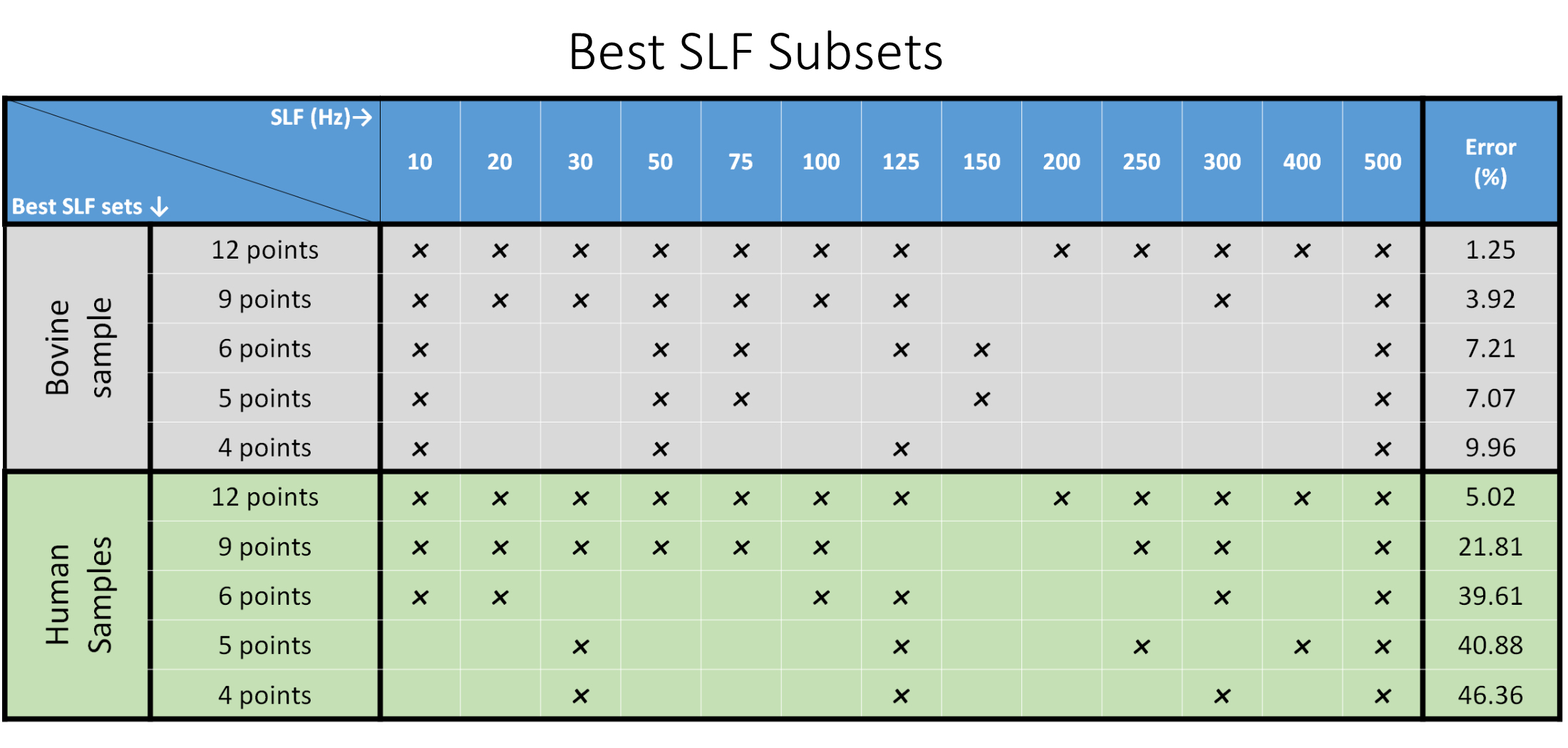
to $$$T_{1\rho}$$$ dispersion data, where ωsl is the SLF, and A, B and $$$\tau_c$$$ are the fitting parameters. Outlier $$$\tau_c$$$ pixels, identified as those with values <1 ms in $$$T_{1\rho}$$$ maps at SLF of 0 Hz calculated from $$$\tau_c$$$ fitting function, were excluded from further analysis. Data analysis was performed using in-house developed MATLAB scripts and plugin functions for Aedes.6 To investigate the role of low and high SLFs on $$$\tau_c$$$ fitting, $$$\tau_c$$$ maps were fitted from different subsets of the $$$T_{1\rho}$$$ dispersion data. Influence of higher SLFs was explored by comparing datasets with different range of SLFs while fixing the lowest SLF (e.g. set1: 10-2500 Hz, set2: 10-2200 Hz,…). Similarly, low SLFs were studied by comparing datasets with different range of SLFs while fixing the highest SLF (e.g. set1: 10-2500 Hz, set2: 20-2500 Hz,...). Resulting $$$\tau_c$$$ maps were evaluated using mean difference and Pearson correlation coefficients with reference $$$\tau_c$$$ map (fitted using full-range dispersion, 10-2500 Hz). To find the optimum distribution of SLFs for $$$\tau_c$$$ fitting in frequency range 10-500 Hz, fitting was applied to data from all possible combinations for 4, 5, 6, 9 and 12 SLFs. Resulting $$$\tau_c$$$ maps were compared pixel-by-pixel with a reference $$$\tau_c$$$ map fitted using all 13 SLFs (10-500Hz). Percentage of absolute mean difference between each tested and reference $$$\tau_c$$$ map for each sample was calculated. Results of both human samples were averaged to form one dataset.
Results
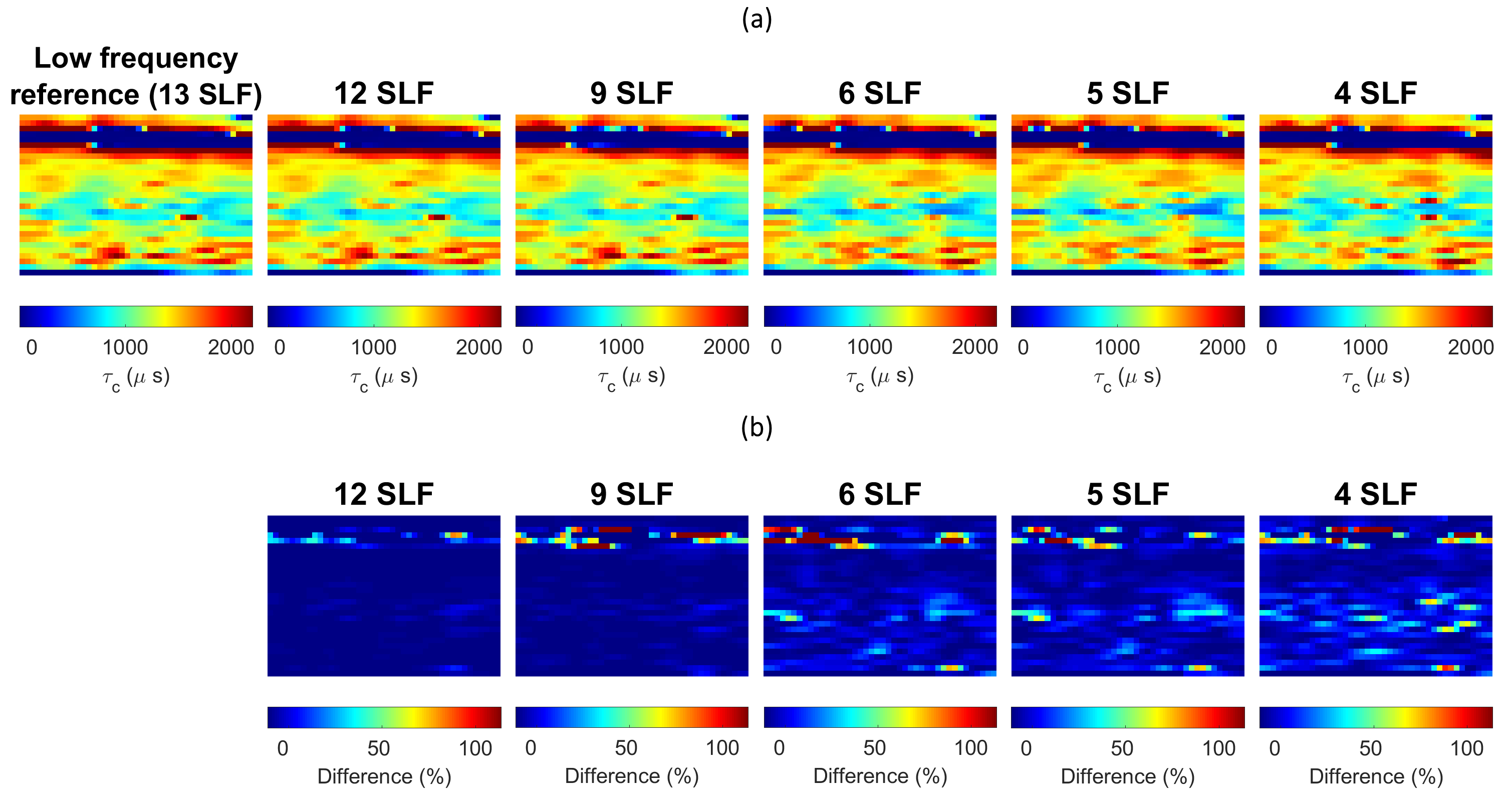
After dropping more than two low-frequency SLFs from the fitting data, correlation of $$$\tau_c$$$ maps with the full-range $$$\tau_c$$$ reference map dropped from 0.63 to -0.10 (Figure 1-a and Figure 2-a). However, even after leaving out 13 high SLFs from fitting, $$$\tau_c$$$ map showed correlation of 0.59 compared to the full-range $$$\tau_c$$$ reference map (Figure 1-b and Figure 2-b). Best selections of 12, 9, 6, 5 and 4 SLFs resulted in $$$\tau_c$$$ maps with mean difference in the range of 1-10% in bovine sample, 5-46% in human samples, compared to the 13 SLFs reference map (Figure 3). $$$\tau_c$$$ maps fitted from best SLFs combinations showed similar laminar appearance to the reference $$$\tau_c$$$ map (Figures 4 and 5).
Discussion and Conclusion
$$$\tau_c$$$ describes $$$T_{1\rho}$$$ dispersion. We infer from the results that SLFs range and selection affect $$$\tau_c$$$ fitting. Less SLFs
generally produces less precise $$$\tau_c$$$ fitting. However, our results show that using
only 6 SLFs results in similar $$$\tau_c$$$ maps as obtained with 13 SLFs. $$$T_{1\rho}$$$ dispersion data for $$$\tau_c$$$ fitting can therefore be obtained in shorter measurement
time without significant loss of information. $$$\tau_c$$$ fitting is
significantly affected by low SLFs while the higher SLFs contribute to a lesser
degree to $$$\tau_c$$$ fitting. In conclusion, although $$$\tau_c$$$ fitting is
sensitive to wide range of molecular processes contributing to $$$T_{1\rho}$$$ relaxation, our
results imply that $$$\tau_c$$$ is more sensitive to molecular processes with
low characteristic frequencies related to dipole-dipole relaxation, or chemical
exchange in cartilage.2,7Acknowledgements
Research funding from Jane and Aatos Erkko Foundation and support from the Academy of Finland (grants #285909 and #293970) are gratefully acknowledged. We also thank CSC-IT Center for Science in Espoo, Finland, for computing time.
References
1. Jones GP. Spin-lattice relaxation in the rotating frame: Weak-collision case. Physical Review. 1966;148(1):332.
2. Sepponen RE, Pohjonen JA, Sipponen JT, Tanttu JI. A method for $$$T_{1\rho}$$$ imaging. J Comput Assist Tomogr. 1985;9(6):1007-1011.
3. Wang P, Block J, Gore JC. Chemical exchange in knee cartilage assessed by $$$R_{1\rho}$$$ (1/$$$T_{1\rho}$$$) dispersion at 3T. Magn Reson Imaging. 2015;33(1):38-42.
4. Nissi MJ, Salo E, Tiitu V, et al. Multi‐parametric MRI characterization of enzymatically degraded articular cartilage. Journal of Orthopaedic Research. 2015.
5. Blicharska B, Peemoeller H, Witek M. Hydration water dynamics in biopolymers from NMR relaxation in the rotating frame. Journal of Magnetic Resonance. 2010;207(2):287-293.
6. Aedes – A graphical tool for analyzing medical images. http://aedes.uef.fi/
7. Mlynarik V, Szomolanyi P, Toffanin R, Vittur F, Trattnig S. Transverse relaxation mechanisms in articular cartilage. Journal of Magnetic Resonance. 2004;169(2):300-307.
Figures
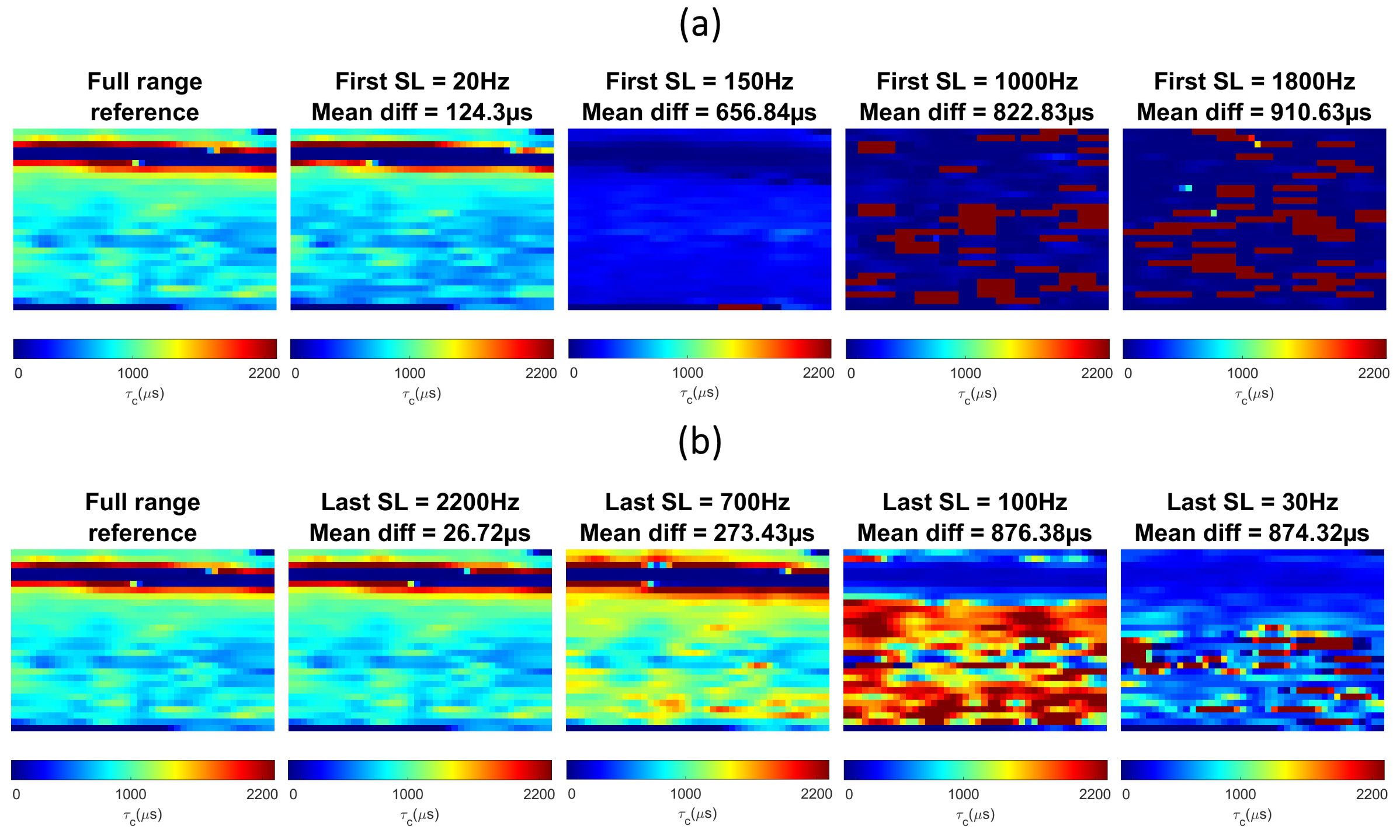
Figure 1: Effect of low and high frequencies SLFs on $$$\tau_c$$$ fitting. (a): $$$\tau_c$$$ ROIs fitted from $$$T_{1\rho}$$$dispersion with lowest SLF increasing from 10 to 1800 Hz. Left ROI is the full-range reference $$$\tau_c$$$ map (SLF range 10-2500 Hz). (b): $$$\tau_c$$$ ROIs fitted from $$$T_{1\rho}$$$dispersion with highest SLF decreased from 2500 to 30 Hz. The mean difference in each map is averaged from its pixel-by-pixel difference with the reference $$$\tau_c$$$ map. Dropping three low frequency SLFs from the fitting data yielded different $$$\tau_c$$$ values than the reference map. However, leaving out 13 high SLFs from fitting resulted in $$$\tau_c$$$ map similar to the reference map.
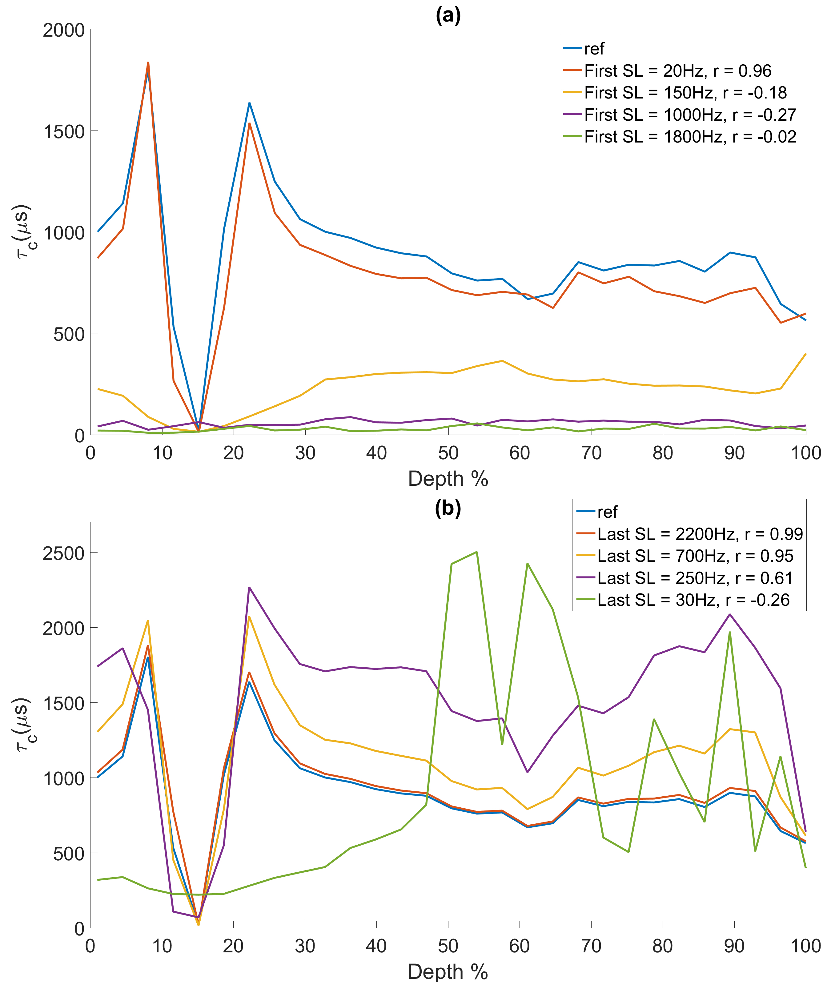
Figure 2: Mean profiles of $$$\tau_c$$$ ROIs in Figure 1 and their correlations with reference map. (a): mean depth wise profiles of each tested $$$\tau_c$$$ map in Figure 1-a plotted vs the reference $$$\tau_c$$$ map profile. Pearson correlation coefficients calculated for the mean profiles. (b): mean depth wise profile of each tested $$$\tau_c$$$ map in Figure 1-b plotted vs the reference $$$\tau_c$$$ map profile. Pearson correlation coefficients calculated for the mean profiles. The correlation decreased significantly, when dropping three or more low frequency SLfs from the fitting data. However, dropping 13 high frequency SLFs yields $$$\tau_c$$$ map with strong correlation to the reference map.