5032
A compact solution for physiological parameters from ultrafast prostate DCE-MRI may reduce random and systematic errors1Radiology, The University of Chicago, Chicago, IL, United States, 2Sino-Dutch Biomedical and Information Engineering School, Northeastern University, Shenyang, China, 3Pathology, The University of Chicago, Chicago, IL, United States
Synopsis
The Tofts pharmacokinetic model requires multiple calculations for analysis of dynamic contrast enhanced (DCE) MRI. This can result in error propagation that reduces the accuracy of pharmacokinetic measurements. Here, we present a new compact solution for estimating physiological parameters based on changes in signal intensity, without the Tofts model. Human prostate DCE-MRI data were analyzed to compare physiological parameters estimated from proposed compact solution with the Tofts model. The Ktrans and ve from the compact solution correlated strongly with values from the Tofts Model. Bland–Altman plots showed moderate to excellent agreement between the compact solution and the Tofts Model.
INTRODUCTION
The Tofts pharmacokinetic model is often used to quantitatively analyze dynamic contrast-enhanced (DCE) MRI data to extract the volume transfer constant (Ktrans) and the contrast media distribution volume (ve).1 This requires calculation of contrast media concentration (C(t)) as a function of time (t), using the ‘full’ non-linear model and accurate measurements of the pre-contrast tissue T1. Therefore, many calculations are required, resulting in error propagation that reduces the accuracy of physiological parameters. In addition, the Tofts compartmental models may not accurately describe the prostate micro-environment, and this can lead to systematic errors. Expanding use of ultrafast DCE-MRI (1-3 seconds/image) allows approximations that can simplify analysis of initial contrast media uptake and avoid the assumptions imposed by pharmacokinetic models. In addition, we can make approximations that simplify analysis of the washout phase. Here, we demonstrate the use of these approximations to produce a compact solution that estimates physiological parameters (Ktrans and ve) based on changes in signal intensity, without the need to fit curves based on the Tofts model.METHODS
The standard Tofts model gives C(t) in tissue following bolus contrast media injection as:1
$$C(t)=K^{trans}\int_{0}^{t} C_p(\tau)\cdot{(-(t-\tau)K^{trans}/v_e)d\tau},---[1]$$
where Cp(t) = Cb(t)/(1-Hct) is the arterial input function (AIF), Cb(t) is contrast media concentration in blood, and Hct is hematocrit (=0.42). At early times after contrast media injection (e.g. t=15 seconds), the efflux of the contrast media from the extravascular extracellular space back to plasma is negligible, and the Eq. [1] can be simplified as (see Patlak model2):
$$C(t)\approx{K^{trans}\int_{0}^{t} {C_p(\tau)d\tau}}.---[2]$$
Then Ktrans can be solved directly or by taking the derivatives on both sides of Eq. [2]:
$$K^{trans}\approx\frac{C(t)}{\int_{0}^{t}{C_p(\tau)d\tau}}\space or\space K^{trans}\approx\frac{1}{C_p(t)}\frac{dC(t)}{dt}, for \space t \ll1.---[3]$$
Using the ‘reference tissue’ model,3 the C(t) can be replaced with the signal intensity S(t), and the integral and derivative formulas become:
$$K^{trans}\approx\frac{\overline{Hct}\cdot{C(t)}}{\int_{0}^{t}{[S_b(\tau)-S_b(0)]d\tau}}\space or\space K^{trans}\approx\frac{\overline{Hct}}{S_b(t)-S_b(0)}\frac{dS(t)}{dt}, for \space t = t_p \ll1,---[4] $$
where $$$\overline{Hct}=1-Hct$$$, Sb(t) is the signal intensity from blood.
To estimate ve, the derivative form of Tofts model was used. At later time (e.g. t >3 minutes) after contrast media injection, we can approximate that $$$dC(t)/dt\approx0$$$, i.e.,:
$$0\approx{K^{trans}[C_p(t)-C(t)/v_e]}\Rightarrow C(t)\approx{v_eC_p(t)}.---[5]$$
Then ve can be estimated from signal intensity:
$$v_e\approx{\overline{Hct}}\frac{S(t)-S(0)}{S_b(t)-S_b(0)}, for\space t = t_N\gg1.---[6]$$
The early time post injection tp was selected as the time-to-peak of the AIF, and tN was the time of the final post-contrast image.
Twenty patients with biopsy-confirmed prostate cancer were enrolled in this IRB-approved study (mean age = 59 years old). MRI data were acquired on a Philips Achieva 3T-TX scanner. After T2-weighted and diffusion-weighted imaging, baseline T1 mapping was performed with variable flip angles. Subsequently, DCE 3D T1-FFE data were acquired pre- and post-contrast media injection (0.1 mmol/kg DOTAREM; TR/TE = 3.5/1.0 ms, FOV = 180×180 mm2, matrix size = 160×160, flip angle = 10°, slice thickness = 3 mm, typical number of slices = 24, SENSE factor = 3.5, half scan factor = 0.625) for 150 dynamic scans with typical temporal resolution of 2.2 sec/image (1.0-4.3 sec).
Regions-of-interest (ROIs) for prostate cancer, normal tissue in different prostate zones and gluteal muscle were drawn on T2W images and transferred to DCE images. ROIs for blood vessels were manually traced on the external femoral artery on a slice with cancer. For each ROI, the average S(t) was calculated, and then C(t) was calculated from the ‘full’ non-linear model.4
RESULTS
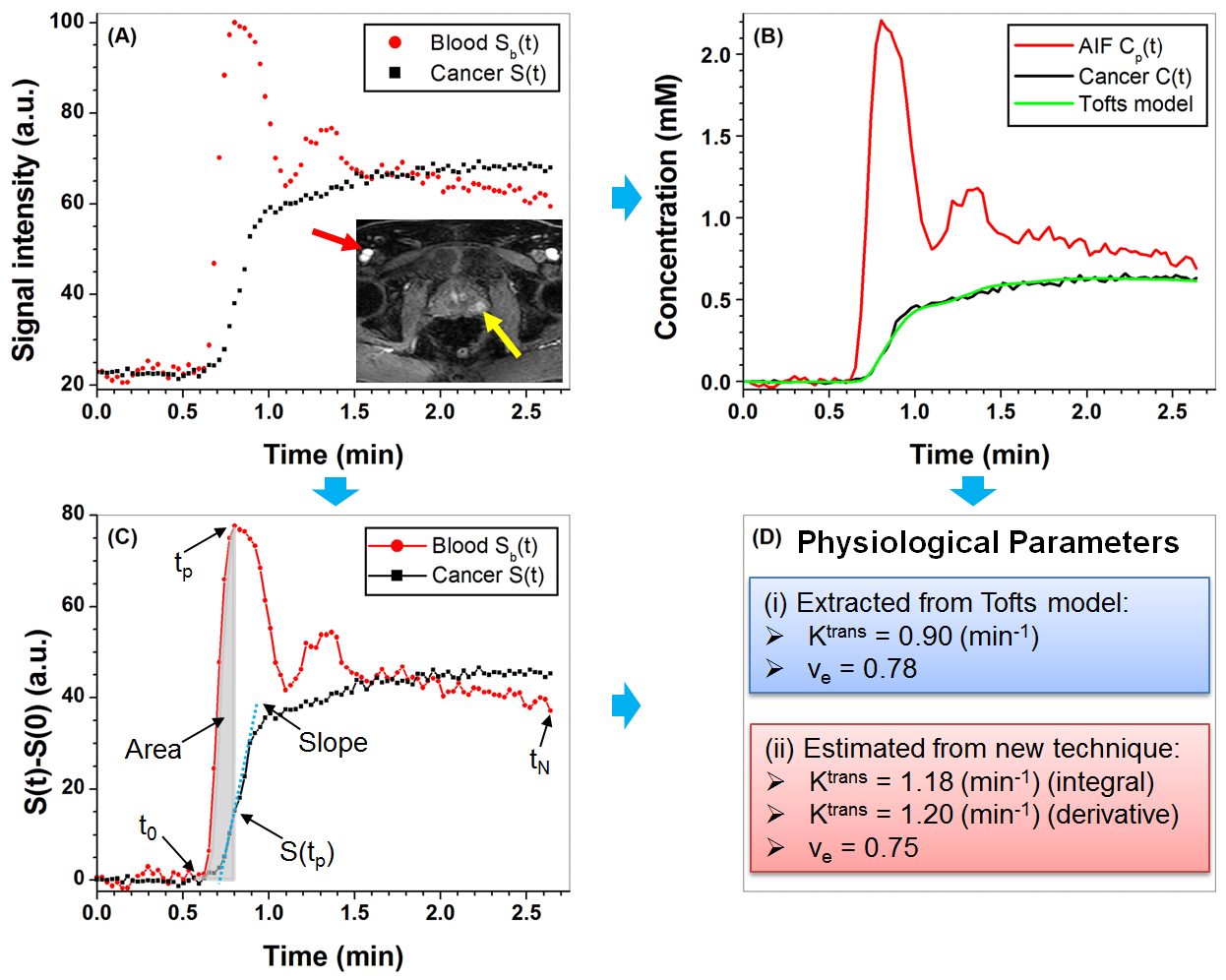
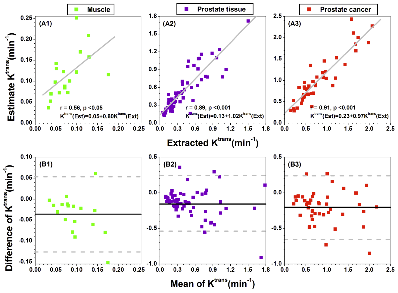
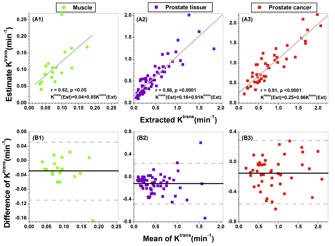
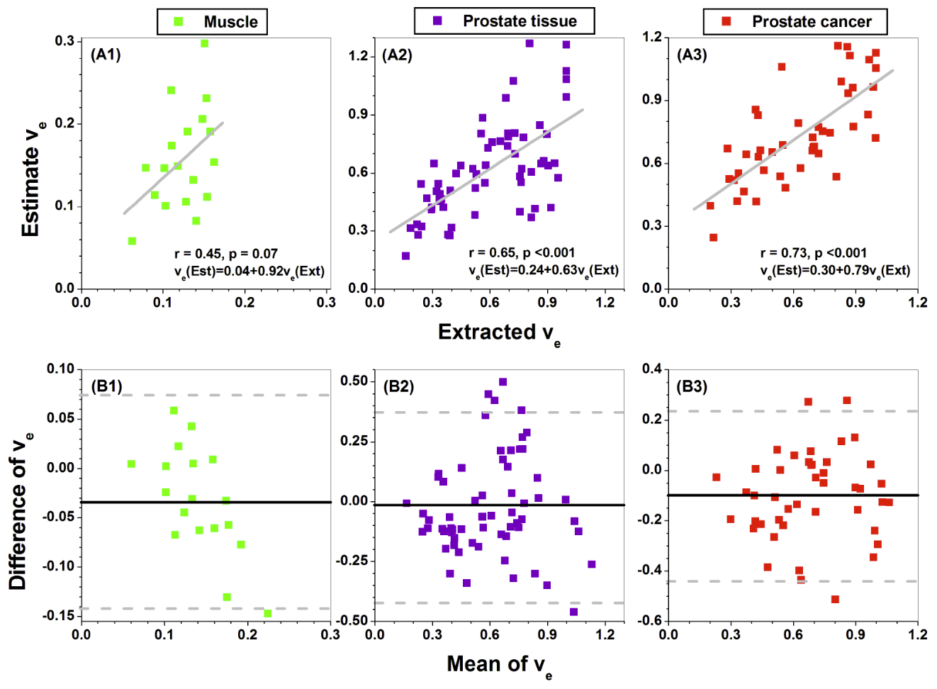
For a typical case, Figure 1 illustrates the steps used to compare estimated and Tofts parameters. Figures 2-4 (A1-A3) show the scatter plots of extracted Ktrans from Tofts model vs. estimated Ktrans from the integral (Fig. 2) and derivative (Fig. 3) formulas, and extracted ve from Tofts model vs. estimated ve (Fig. 4) for different ROIs. There was strong (r=0.88 to 0.91, p<0.0001) positive correlations between the Tofts Ktrans and estimated Ktrans for prostate cancer and normal tissue. There was moderate correlation between Tofts ve and estimated ve (r=0.65 to 0.73, p<0.0001). The corresponding Bland–Altman plots (Figures 2-4 (B1-B3)) show moderate to excellent agreement between Tofts and estimated physiological parameters.DISCUSSION
Human prostate DCE-MRI data were used to validate our compact method for estimation of physiological parameters. Overall agreement between values from the compact solution and Tofts model values was very good. Sensitivity and specificity of the new method was not tested here, but we hypothesize that the compact calculation reduces propagation of random error. Furthermore, use of the compact solution may decrease systematic error due to use of pharmacokinetic models that do not accurately describe the micro-environment of normal prostate and prostate cancer. We are currently performing a clinical trial to test this hypothesis.Acknowledgements
This research is supported by Guerbet LLC, Philips Healthcare, and National Institutes of Health (R01 CA172801-01, R01 CA218700-01, and 5U01 CA142565-09).References
1. Tofts PS, Brix G, Buckley DL, et al. Estimating kinetic parameters from dynamic contrast-enhanced T(1)-weighted MRI of a diffusable tracer: standardized quantities and symbols. J Magn Reson Imaging 1999;10:223-32.
2. Patlak CS, Blasberg RG. Graphical Evaluation of Blood-To-Brain Transfer Constants from Multiple-Time Uptake Data - Generalizations. Journal of Cerebral Blood Flow and Metabolism 1985;5(4):584-90.
3. Medved M, Karczmar G, Yang C, et al. Semiquantitative analysis of dynamic contrast enhanced MRI in cancer patients: Variability and changes in tumor tissue over time. J Magn Reson Imaging 2004;20(1):122-128.
4. Dale BM, Jesberger J A, Lewin JS, et al.. Determining and optimizing the precision of quantitative measurements of perfusion from dynamic contrast enhanced MRI. J Magn Reson Imaging 2003;18:575-84.
Figures