5028
Is the Parker arterial input function necessary to model the second pass for dynamic contrast enhanced MRI? - A simulation study1Sino-Dutch Biomedical and Information Engineering School, Northeastern University, Shenyang, China, 2Radiology, The University of Chicago, Chicago, IL, United States
Synopsis
Accurately modeling arterial input function (AIF) is important for dynamic contrast enhanced (DCE) MRI. Simulations were performed comparing nine population AIF models to the Parker AIF. Effects of AIF second pass with and without adding noise onto extracted physiological parameters were evaluated with n=1,000 randomly generated physiological parameters (Ktrans and ve) used to calculate contrast agent concentration curves using the Tofts model and Parker AIF. Results demonstrated that the six-parameter linear function plus bi-exponential function AIF model was almost equivalent to Parker AIF. Effects of the second pass were small, unless noise with signal-to-noise ratio was <10 dB.
INTRODUCTION
Physiological parameters (Ktrans and ve) extracted from pharmacokinetic models rely on accurate arterial input functions (AIF). Reliable AIFs are not easily obtained and sometimes cannot be measured from a specific dynamic contrast enhanced (DCE) MRI protocol. Therefore, it often relies on a population AIF, which is exhibited in mathematical form. Although Parker AIF model is relatively widely used,1 it’s not always the best model to fit measured AIF with noise. The Parker model was less robust to fit measured AIF, unless the initial guesses are similar to actual values. If the second pass is much smaller than the first pass and less important, then the AIF models could be simplified. Here numerical simulations were used to evaluate which nine mathematical AIF models with a small number of parameters were most similar to the Parker model. The effects of the second pass of Parker AIF model with and without adding noise on extracted Ktrans and ve were evaluated by using a simple mathematical AIF model without the second pass.METHODS
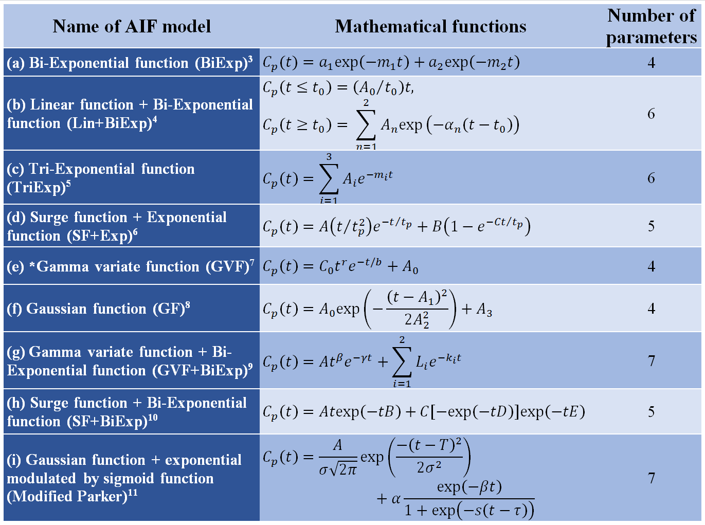
There are 10 parameters in Parker model: An, Tn, and σn (n = 1, 2) are the scaling constant, center, and width of the Gaussian, respectively; α and β are the amplitude and decay constant of the exponential; and s and τ are the width and center of the sigmoid. The Parker AIF (Cp(t)) was calculated with average parameters, 1.5 seconds temporal resolution, and sampled for 6 minutes. Then, the other nine population AIF models (Table 1) were used to fit the Parker AIF model. The closest model to Parker model with the smallest number of parameters was selected to study the second pass effects of AIF.
To maximize the second pass, a new Parker AIF (Cp2(t)) was calculated by setting parameters so that the first pass peak is lower and the second pass peak is higher and wider. Therefore, Parker’s average parameters were set to be plus or minus 2.58 times standard deviations (SD): A1 and T1 were set to be mean-2.58*SD; A2, T2, σ2, α and β were set to be mean+2.58*SD; and σ1, s and τ were kept as mean values. As result, new AIF had ratios of A2/A1=0.62 and σ2/σ1=3.31, which were much larger than the AIF calculated with average parameters.
The following steps were used in the computer simulations for a total of 1,000 contrast agent concentration curves C(t):
(i) Random numbers (rn1 and rn2) uniformly distributed between 0 and 1 were generated and mapped into the following interval to obtain practical Ktrans and ve values:
$$K^{trans}=0.05+r_{n1}\cdot(1.0-0.05),v_e=0.05+r_{n2}\cdot(0.75-0.05).$$
To be more realistic, only values of Ktrans and ve such that Ktrans/ve < 10 were used in the simulations. Then C(t) was calculated by using Tofts model with new Cp2(t):2
$$C(t)=K^{trans}\int_{0}^{t} C_{p2}(\tau)\cdot exp(-K^{trans}(t-\tau)/v_{e})d\tau.$$
(ii) The simple AIF with the smallest number of parameters close to Parker AIF was used to fit the C(t) to extract Ktrans and ve values and compared with generated values. The effect of noise on Cp2(t) was also studied by adding white Gaussian noise with signal to noise ratio (SNR) of 10, 5, and 1 dB.
RESULTS
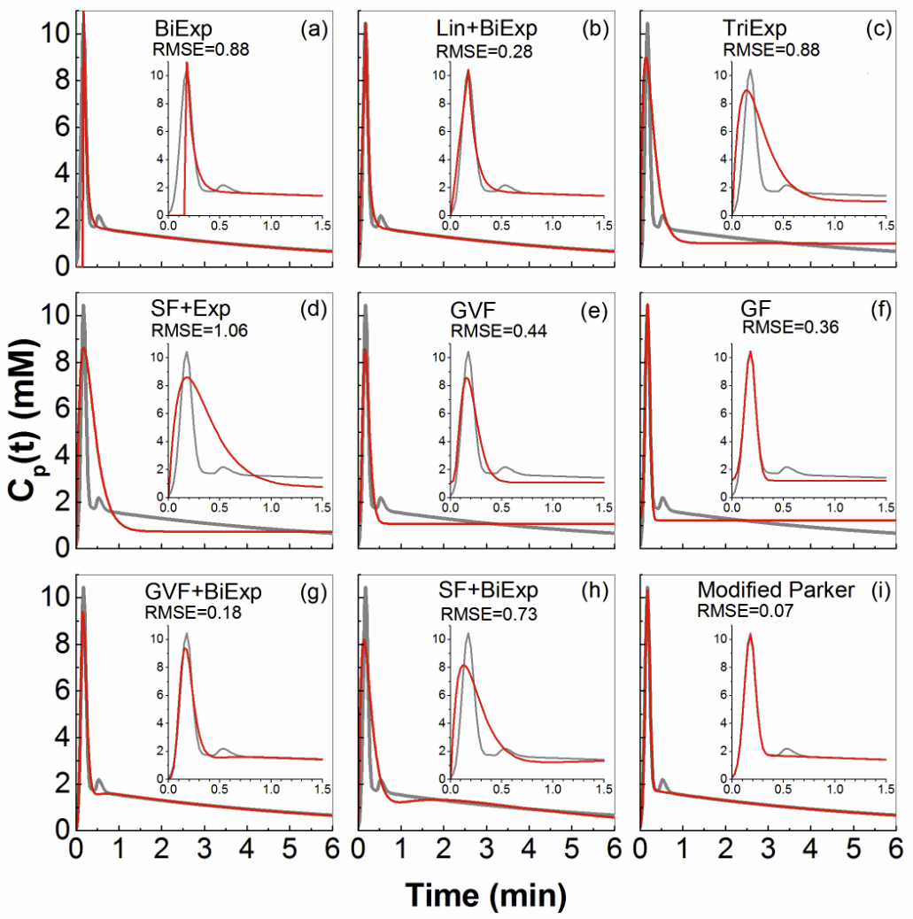
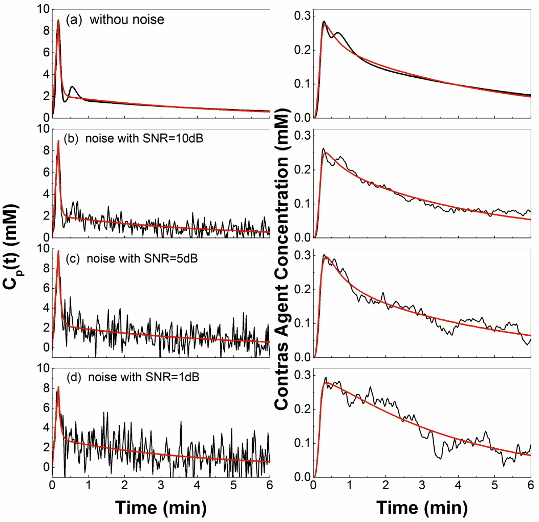
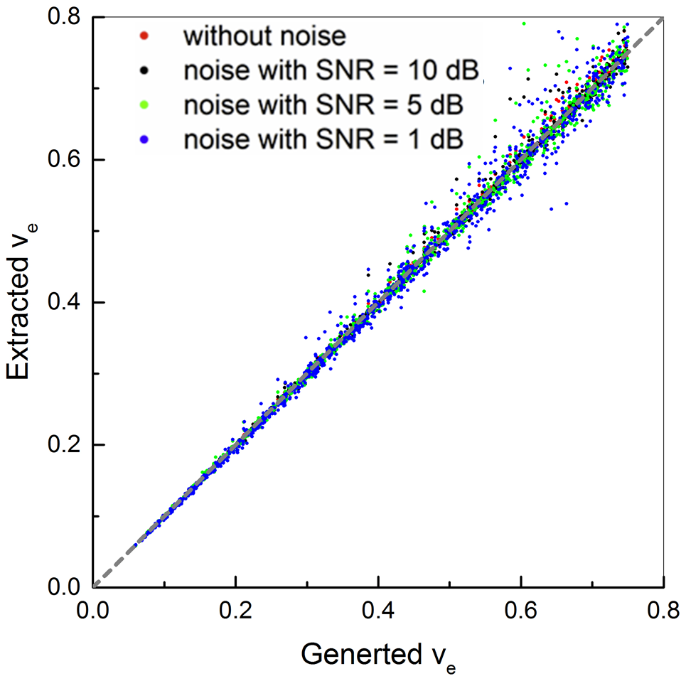
Figure 1 shows plots of Parker AIF (gray line) and corresponding fits (red line) obtained from nine AIF models (a–i) listed in Table 1. Obviously, the Lin+BiExp, GVF+BiExp, and modified Parker models fit best, and the Lin+BiExp have the smallest number of parameters. Figure 2 (a–d) left panel shows the Lin+BiExp model fits (red lines) to Cp2(t) (black lines) with added white Gaussian noise, and right panel shows the corresponding calculated C(t). Figures 3 and 4 show scatter plots of generated vs. extracted Ktrans and ve from the Lin+BiExp model, respectively. Without modeling the second pass of AIF (noise free), the extracted Ktrans was about 3% underestimated than generated Ktrans. On average, the extracted Ktrans was about 10%, 15% and 20% underestimated than the generated Ktrans for SNR = 10, 5, and 1 dB, respectively. The second pass and added noise had much smaller effects on extracting ve.DISCUSSION
Our study is based on reviewing and summarizing the previous work published regarding the AIF models. We demonstrated that the Lin+BiExp AIF model was almost equivalent to the Parker AIF. The Lin+BiExp model was much more robust to fit measured AIF because of the smaller number of parameters and the absence of Gaussian functions. The effects of the second pass of contrast agent circulation were small on extracted physiological parameters using the Tofts model, unless noise was added with signal to noise ratio less than 10 dB.Acknowledgements
The research is supported by the National Natural Science Foundation of China (No. 61672146) and the 2011 Collaborative Innovation Program of Guizhou Province (2015-04). We would like to thank Ms. Erica Markiewicz for carefully reading the abstract.References
1. Parker GJ, Roberts C, Macdonald A, et al. Experimentally-derived functional form for a population-averaged high-temporal-resolution arterial input function for dynamic contrast-enhanced MRI. Magn Reson Med 2006;56(5):993-1000.
2. Tofts PS, Brix G, Buckley DL, et al. Estimating kinetic parameters from dynamic contrast-enhanced T(1)-weighted MRI of a diffusable tracer: standardized quantities and symbols. J Magn Reson Imaging 1999;10:223-32.
3. Tofts PS, Kermode AG. Measurement of the blood-brain barrier permeability and leakage space using dynamic MR imaging. 1. Fundamental concepts. Magn Reson Med 1991;17(2):357-367.
4. Su MY, Jao JC, Nalcioglu O. Measurement of vascular volume fraction and blood-tissue permeability constants with a pharmacokinetic model: studies in rat muscle tumors with dynamic Gd-DTPA enhanced MRI. Magn Reson Med 1994;32(6):714-724.
5. Tofts PS. Modeling tracer kinetics in dynamic Gd-DTPA MR imaging. J Magn Reson Imaging 1997;7(1):91-101.
6. Simpson NE, He Z, Evelhoch JL. Deuterium NMR tissue perfusion measurements using the tracer uptake approach: I. Optimization of methods. Magn Reson Med 1999;42(1):42-52.
7. Calamante F, Gadian DG, Connelly A. Delay and dispersion effects in dynamic susceptibility contrast MRI: simulations using singular value decomposition. Magn Reson Med 2000;44(3):466-473.
8. Mlynash M, Eyngorn I, Bammer R, et al. Automated method for generating the arterial input function on perfusion-weighted MR imaging: validation in patients with stroke. AJNR Am J Neuroradiol 2005;26(6):1479-1486.
9. Workie DW, Dardzinski BJ. Quantifying dynamic contrast-enhanced MRI of the knee in children with juvenile rheumatoid arthritis using an arterial input function (AIF) extracted from popliteal artery enhancement, and the effect of the choice of the AIF on the kinetic parameters. Magn Reson Med 2005;54(3):560-568.
10. Yankeelov TE, Luci JJ, Lepage M, et al. Quantitative pharmacokinetic analysis of DCE-MRI data without an arterial input function: a reference region model. Magn Reson Imaging 2005;23(4):519-529.
11. McGrath DM, Bradley DP, Tessier JL, et al. Comparison of model-based arterial input functions for dynamic contrast-enhanced MRI in tumor bearing rats. Magn Reson Med 2009;61 (5):1173-1184.
Figures