5022
Investigating the nature of distinct regions in brain tissue affected by stroke with principal component analysis of multi-b valued diffusion data1Institute of Neuroscience and Medicine 4, Medical Imaging Physics, Research Centre Juelich, Juelich, Germany, 2Department of Neurology, Faculty of Medicine, RWTH Aachen University, Aachen, Germany
Synopsis
A data-driven, observer-independent segmentation of brain regions affected by stroke is proposed. It is based on PCA analysis of a multi b-value diffusion trace acquisition and offers fast, high-SNR visualisation of affected areas. Substructure of these areas is easily identified and can be automatically delineated using clustering algorithms.
Purpose
One of the biggest remaining problems in stroke treatment is determining the precise time of stroke and precise areal affected by it [1-4]. There is evidence that high b value DWI could detect more ischemia lesions than conventional one [5–11], as also substantiated by findings based on diffusion kurtosis [e.g 12] and q-space imaging [13]. High-b-value information appears thus complementary to the typical DWI at b=1000 s/mm2. At the other end of diffusion weighting, perfusion studied with diffusion methods (IVIM, [14]) is enjoying a strong come-back in clinical stroke [15-17].
We have designed a protocol which combines information about perfusion, ADC changes, kurtosis and q-space from the same set of 16 diffusion trace acquisitions, with b-values covering the range between 0 and 10,000 s/mm2 and applied it to measurements on stroke patients (TA=6min:53). Whereas it is possible to extract quantitative parameters characterising the three diffusion regimes (ultra-fast, fast and slow) from this data set, we concentrate here on describing a computationally cheap and very fast method to visualise the information obtained from the full acquisition with very high SNR and sensitivity using Principal Component Analysis (PCA).
Methods
Data from eight stroke patients (5 male, 3 female, mean age 67.78 yrs, from 52 to 79) were included in this study, covering the time range between hyperacute (3hrs) and subacute (8 days) stroke with a mean of 3.8 days post symptom onset. Informed consent was obtained from all patients and the measurements were conducted in agreement with the requirements of the local ethics committee. All experiments were run on a 3T PRISMA scanner (Siemens Medical Solutions, Erlangen, Germany) equipped with 80mT/m gradients, using a body coil for signal transmission and a 20-channel head receiver coil. Diffusion data were acquired with the manufacturer’s trace DWI protocol. Sixteen unevenly spaced b-values were acquired, from 0 to 10,000 s/mm2 with total acquisition time 6:53 min. The dataset was split for further processing into a “low b” group of 7 values (0-1500 s/mm2) and a “high b” group of 9 values (2000-10000 s/mm2) reflecting different diffusion regimes. PCA analysis was done in Matlab separately for each b-value group. Clustering analysis based on a k-means algorithm was performed on 5 principal components (3 from low b-values, 2 from high b-values) shown in Fig. 1. In addition to the PCA-based analysis, ADC and apparent kurtosis indices were obtained by fitting the relevant range of b values (0, 1000, 1500, 2000, 3000) and changes caused by stroke in these indices were assessed. Masks of the affected area were independently drawn by an experienced neuroradiologist based on standard DWI and FLAIR information.Results and Discussion
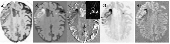
The
properties of eigenvectors and eigenvalues (Fig. 2a and 2b, respectively)
obtained by the PCA analysis were found to be remarkably consistent for all 8
patients, and independent of the size of the lesion. The visualisation of the
lesion in each distinct component was also very similar between patients.
Affected
areas were visualised with very high (positive or negative) contrast in all 5
selected components. The lesion-to-brain
intensity ratio reached values from 3 to above 10 for individual voxels. In
comparison, ADC effects are of the order of 30%, kurtosis of the order of 50%.
Very clearly, the features of the conspicuous area are reflected differently by
each component.
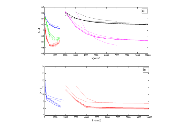
The
results of k-means clustering for one patient are shown in Fig. 3a for a
selected slice, to be compared to the mask defined manually (Fig. 3b).
The
manually drawn mask includes voxels from at least 4 “lesion clusters” which are
presumably distinct in their diffusion and perfusion properties.
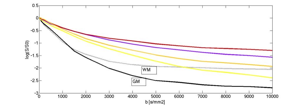
In order
to investigate the diffusion properties of the voxels from each cluster, an
averaged decay curve per cluster is plotted in Fig. 4 together with curves from
selected WM and GM regions. It is thus apparent that all clusters in the stroke
region have slower decay than normal tissue, but differ in the degree of and
component affected by changes (perfusion, fast and slow diffusion).
A
quantitative description of the properties of each cluster based on multi-component
fitting and comparison between patients is in progress.
The exact
nature of these regions remains to be further investigated, for example by
following their progression in longitudinal studies and measuring additional
parameters such as standard perfusion, water content, NMR relaxation times. It
is to be expected that characterising changes caused by stroke in each of these
clusters separately might lead to better trend definition and eventually better
understanding of the effects of stroke on tissue microscopy.Acknowledgements
No acknowledgement found.References
1. Attyé, A, Boncoeur-Martel MP,. Maubon A et al.: Diffusion-Weighted Imaging infarct volume and neurologic outcomes after ischemic stroke. In: J Neuroradiol 2012;2:97-103
2. Olivot JM & Marks MP, Magnetic resonance imaging in the evaluation of acute stroke.Top Magn Reson Imaging 2008;5:225-230
3. Wintermark M, Flanders AE, Velthuis B, et al. Perfusion-CT Assessment of Infarct Core and Penumbra, Receiver Operating Characteristic Curve Analysis in 130 Patients Suspected of Acute Hemispheric Stroke. 2006;37:979-85
4. Thomalla G, Cheng B, Ebinger M, et al. DWI-FLAIR mismatch for the identification of patients with acute ischaemic stroke within 4·5 h of symptom onset (PRE-FLAIR): a multicentre observational study Lancet Neurol. 2011;10:978-86
5. Lettau M, Laible M. 3-T high-b-value diffusion-weighted MR imaging in hyperacute ischemic stroke. J Neuroradiol. 2013;40:149–157. doi: 10.1016/j.neurad.2012.08.007.
6. Purroy F, Begue R, Quílez A, Sanahuja J, Gil MI. Contribution of high-b-value diffusion-weighted imaging in determination of brain ischemia in transient ischemic attack patients. J Neuroimaging. 2013;23:33–38. doi: 10.1111/j.1552-6569.2011.00696.x.
7. Cihangiroglu M, Citci B, Kilickesmez O, Firat Z, Karlıkaya G, Uluğ AM, Bingol CA, Kovanlikaya I. The utility of high b-value DWI in evaluation of ischemic stroke at 3T. Eur J Radiol. 2011;78:75–81. doi: 10.1016/j.ejrad.2009.10.011.
8. Lettau M, Laible M. 3-T high-b-value diffusion-weighted MR imaging of hyperacute ischemic stroke in the vertebrobasilar territory. J Neuroradiol. 2012;39:243–253. doi: 10.1016/j.neurad.2011.09.005.
9. Burdette JH, Elster AD. Diffusion-weighted imaging of cerebral infarctions: Are higher B values better? J Comput Assist Tomogr. 2002;26:622–627. doi:10.1097/00004728-200207000-00026.
10. Meyer JR, Gutierrez A, Mock B, Hebron D, Prager JM, Gorey MT, Homer D. High-b-value diffusion-weighted MR imaging of suspected brain infarction. AJNR Am J Neuroradiol. 2000;21:1821–1829.
11. Kim HJ, Choi CG, Lee DH, Lee JH, Kim SJ, Suh DC. High-b-value diffusion-weighted MR imaging of hyperacute ischemic stroke at 1.5T. AJNR Am J Neuroradiol. 2005;26:208–215
12. Hui ES, Fieremans E, Jensen JH, et al. Stroke Assessment with Diffusional Kurtosis Imaging. Stroke; a journal of cerebral circulation. 2012;43(11):2968-2973. doi:10.1161/STROKEAHA.112.657742.
13. Hori M, Motosugi U, Fatima Z, et al. A comparison of mean displacement values using high b-value q-space diffusion-weighted MRI with conventional apparent diffusion coefficients in patients with stroke. Acad Radiol 2011; 18:837–841.
14. Le Bihan D, Breton E, Lallemand D, Aubin ML, Vignaud J, Laval-Jeantet M. Separation of diffusion and perfusion in intravoxel incoherent motion MR imaging. Radiology. 1988 Aug;168(2):497-505.
15. C. Federau, S. Sumer, F. Becce, P. Maeder, K. O’Brien, R. Meuli. Intravoxel incoherent motion perfusion imaging in acute stroke: initial clinical experience. Neuroradiology 2014; 56:629-635
16. Suo S et al., Stroke assessment with intravoxel incoherent motion diffusion-weighted MRI. NMR Biomed 2016; 29:320-8
17. Yao Y, Zhang S, Tang X, Zhang S, Shi J, Zhu W, Zhu W. Intravoxel incoherent motion diffusion-weighted imaging in stroke patients: initial clinical experience. Clin Radiol 2016; 71:938
Figures