5001

Reducing Streaking Artifacts in Quantitative Susceptibility Mapping via Deep Learning

Jie Liu¹, Yida Wang¹, Yang Song¹, Haibin Xie¹, Jianqi Li¹, and Guang Yang¹

¹Shanghai Key Laboratory of Magnetic Resonance, East China Normal University, Shanghai, China

Synopsis

In this study, we proposed a new approach to reduce streaking artifacts in quantitative susceptibility mapping via deep learning. It combined two convolutional neural networks to reduce streaking artifacts from classic threshold-based k-space division (TKD) . The proposed method achieved impressive performance both visually and statistically.

Purpose

In recent years, quantitative susceptibility mapping (QSM) has been developed as a novel MR technique to assess brain iron in vivo. However, QSM is an ill-conditioned inverse problem in calculating underlying magnetic susceptibility distribution from phase image. Threshold-based k-space division (TKD)¹ is a direct method to solve this problem without explicit a priori knowledge. However, it suffers from severe streaking artifacts. Inspired by the recent achievements of deep learning in medical imaging, we proposed a two-stage convolutional neural network (CNN) to reduce streaking artifacts in QSM images. Firstly, we used a simple CNN to remove major artifacts in images produced by TKD; then another network with U-net architecture² was used to learn structure information of images.

Theory

The relationship between measured phase map and underlying susceptibility distribution can be expressed as $$ \delta\left(k\right) = D\left(k\right)\cdot\chi\left(k\right)\\ \\ \delta\left(k\right)= \frac{\phi\left(k\right)}{ 2\pi\cdot\gamma\cdot H_{0} \cdot TE} \qquad D\left(k\right)=\frac{1}{3}-\frac{k_{z}^{2}}{k^{2}} $$ where $$$ \gamma$$$, $$$H_{0}$$$, and $$$ TE$$$ denote gyromagnetic ratio, applied magnetic field and echo time, respectively. $$$\phi\left(k\right)$$$, $$$D\left(k\right)$$$, $$$\delta\left(k\right)$$$ and $$$\chi\left(k\right)$$$ denote the Fourier transform of phase image, dipole kernel, normalized field map, and susceptibility distribution, respectively. To reduce the artifacts in the susceptibility map, we substitute $$$\chi\left(k\right)$$$ with the output of CNN in k-space wherever $$$\left\|D\left(k\right)\right\|$$$ is smaller than a certain threshold t, namely: $$ \chi\left(k\right)= \begin{cases} \chi^{'}_{recon.}\left(k\right) \qquad \left\|D\left(k\right)\right\|<t \\ \\ \chi_{ori.}\left(k\right)=\frac{\delta\left(k\right)}{D\left(k\right)} \ otherwise \end{cases} $$ Where $$$\chi_{ori.}\left(k\right)$$$ and $$$ \chi^{'}_{recon.}\left(k\right)$$$ represent the original susceptibility map and reconstructed results in k-space from two stage networks, respectively.

Methods

We took a 3D simulated model of the brain³ as the true susceptibility distribution. The phase image $$$\phi\left(r\right)$$$ was synthesized by forward model⁴, where TE = 26ms, B₀ = 3T, voxel size = 0.5mm$$$\times$$$0.5mm$$$\times$$$0.5mm and matrix size = 640$$$\times$$$640$$$\times$$$640. An initial estimation of the susceptibility map with streaking artifacts was reconstructed from phase image by TKD where truncated value t = 0.1 was used¹. Since deep learning requires a large amount of samples to achieve satisfactory results, we augmented the data by rotating the brain image for different angles in 3D before synthesizing phase images. 1400 and 200 QSM 2D images were used for training and testing respectively, each cropped to 400$$$\times$$$400.

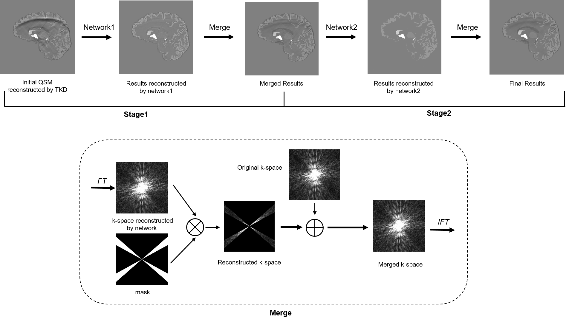
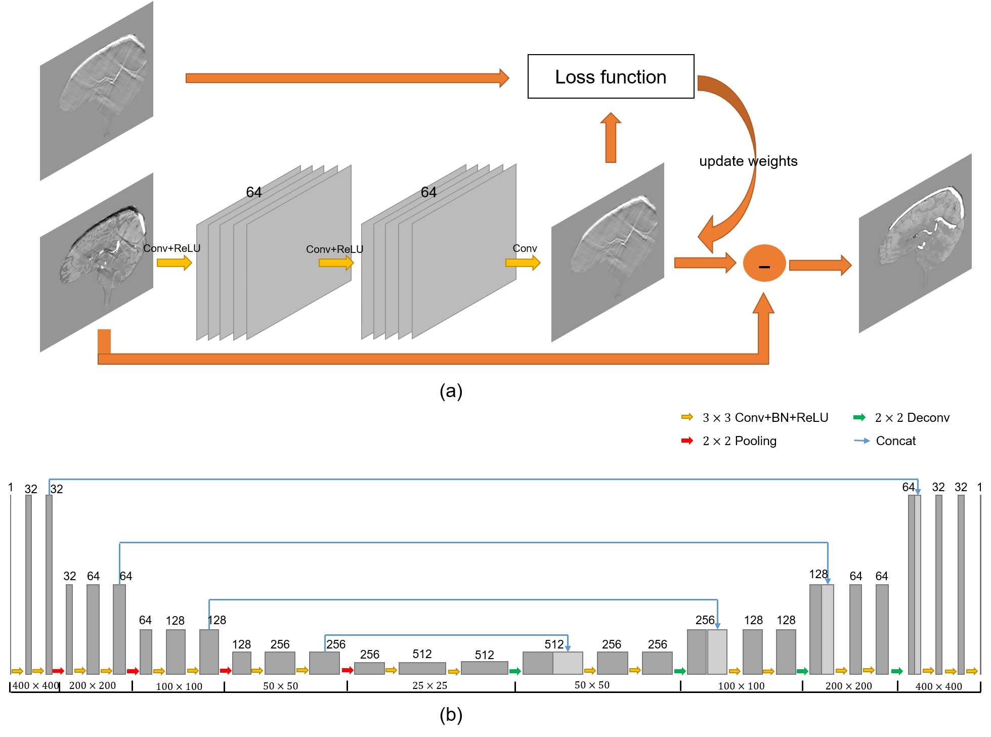
The flowchart of the proposed two-stage method is shown in Fig. 1. In the first stage, QSM images with streaking artifacts were input into the trained network1 as shown in Fig. 2(a) to get the artifacts images. Then, we obtained artifacts-free images by subtracting the artifacts images from QSM images with streaking artifacts. Then the Fourier-transformed artifacts-free images $$$\chi^{'}_{recon.}\left(k\right)$$$ was merged with original k-space $$$\chi_{ori.}\left(k\right)$$$. Finally, the merged k-space was inverse Fourier transformed to get the reconstructed images of the first stage. In the second stage, we used a U-net architecture network as shown in Fig. 2(b) to learn the end-to-end mapping from reconstructed images of the first stage to ground truth. Then we merged the k-space data to obtain the final reconstructed images.

During the training, we used stochastic gradient descent (SGD) to minimize the loss function (Euclidean distance function). Our CNN model was built with TensorFlow, and run on a personal computer powered with two NVIDIA Titan X GPUs for about 24 hours on training. It took only tens of milliseconds to reconstruct single slice image.

Results and Discussion

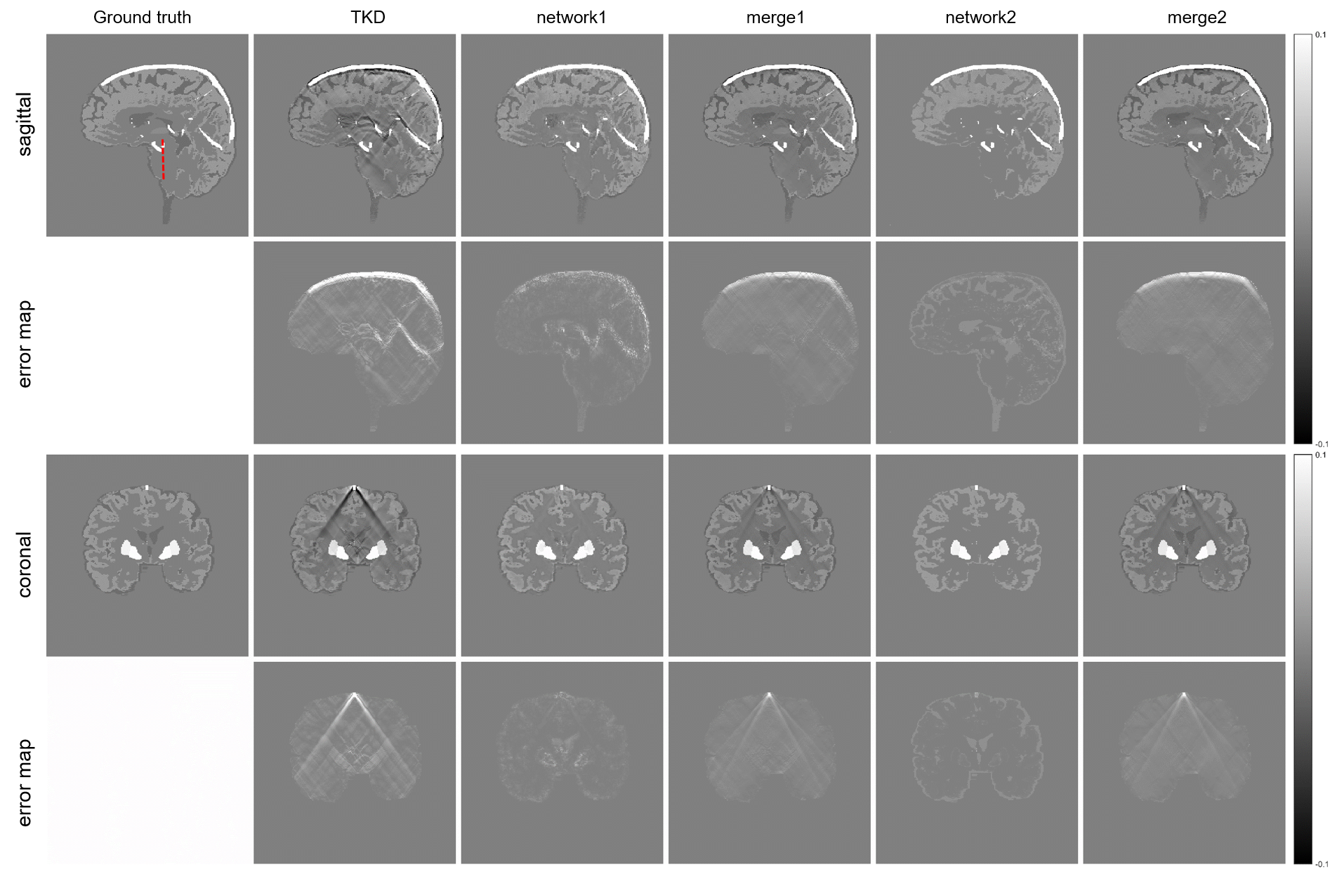
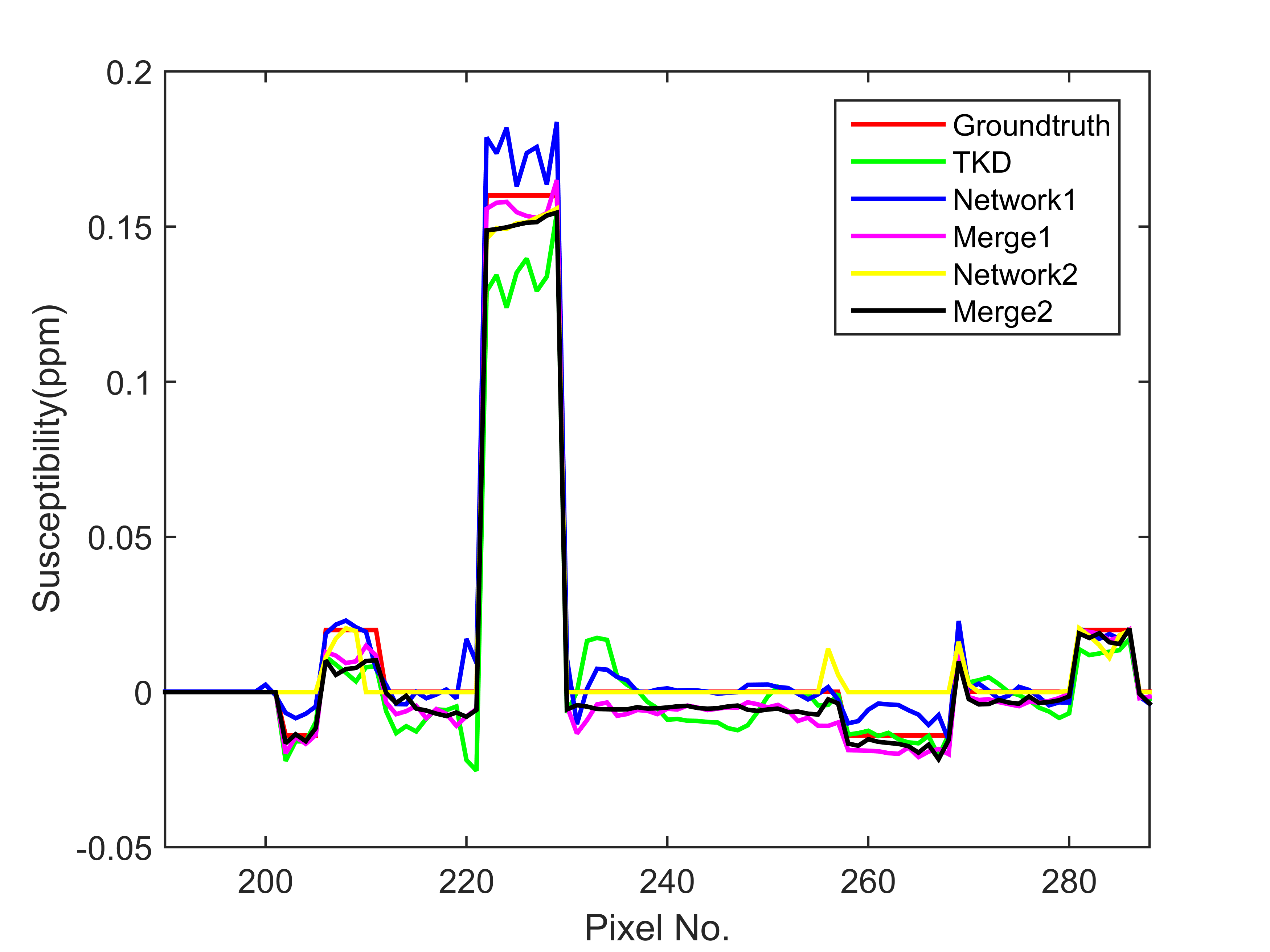
The reconstructed results of the proposed method are shown in Fig. 3. Compared to the TKD method, network 1 significantly reduces streaking artifacts, but some structure information is lost. K-space merging recovers structural details but brings back some artifacts. So we used network 2 to further reduce artifacts. Artifacts in the regions where tissue has high susceptibility values, which are very obvious in merge 1 images, are mostly removed in merge 2 images. (Fig. 3). In addition, merge 2 results is closer to the true susceptibility profile compared with other results in the low susceptibility regions (Fig. 4).

Conclusion

In this study, we used two CNN networks of different structures to reconstruct QSM images. According to the experimental results, the proposed method can significantly reduce streaking artifacts and preserve image details at the same time, and thus can effectively improve the image quality.

Acknowledgements

The study was supported by the key project of the National Natural Science Foundation of China (61731009). The authors would like to thank Dr. Sagar Buch and Dr. E. Mark Haacke for their discussion about the 3D brain model.

References

1. Wharton S, Schafer A, Bowtell R. Susceptibility mapping in the human brain using threshold-based k-space division. Magn Reson Med 2010;63:1292–1304.

2. Ronneberger O, Fischer P, Brox T. U-Net: convolutional networks for biomedical image segmentation. International Conference on Medical Image Computing and Computer-Assisted Intervention. Springer, Cham, 2015:234-241.

3. Buch S, Liu S, Neelavalli J, et al. Simulated 3D brain model to study the phase behavior of brain structures. In: Proceedings of the International Society for Magnetic Resonance in Medicine 20th Scientific Meeting, 2012; Melbourne, Australia. p. 2332.

4. Marques J, Bowtell R. Application of a Fourier-based method for rapid calculation of field inhomogeneity due to spatial variation of magnetic susceptibility. Concept Magn Reson B 2005;25B:65–78.

Figures

Figure 1. The flowchart of the proposed method. The process of merging data is shown in the dotted box below.

Figure 2. (a) Network1 includes 3 convolution layers and 2 ReLU(Rectified Linear Unit) layers. (b) Network2 with U-net architecture, consists of convolution (Conv), batch normalization (BN), ReLU and concatenation(Concat) layers. Pooling and deconvolution layers are applied to increase the depth of the network. The numbers and scales of feature maps are displayed at the top and bottom, respectively.

Figure 3. Reconstructed results of the proposed method. The top two rows show the reconstructed susceptibility map $$$\chi\left(r\right)$$$ and corresponding error map $$$\|\chi\left(r\right)-\chi_{gt}\left(r\right)\|$$$ in sagittal view; the bottom two rows show reconstructed results in a coronal view.

Figure 4. Susceptibility proﬁles of red line in Fig. 3 with different reconstructed results.

Proc. Intl. Soc. Mag. Reson. Med. 26 (2018)

5001