4999
A multi-scale approach to quantitative susceptibility mapping (MSDI)1Wellcome Centre for Human Neuroimaging, UCL Insitute of Neurology, University College London, London, United Kingdom, 2Department of Electrical Engineering, Pontificia Universidad Catolica de Chile, Santiago, Chile, 3Biomedical Imaging Center, Pontificia Universidad Catolica de Chile, Santiago, Chile
Synopsis
We propose a new QSM algorithm, namely multi-scale dipole inversion (MSDI), which builds on the nonlinear MEDI (nMEDI) framework incorporating two additional features: (i) improved error control through dynamic phase-reliability compensation across harmonic scales and (ii) scale-specific use of the morphological prior. MSDI is the first algorithm to rank in the top-10 for all performance metrics evaluated in the 2016 QSM Reconstruction Challenge. It also demonstrates lower variance than nMEDI in a reproducibility test.
Purpose
To develop a multi-scale QSM algorithm extending the nMEDI framework1 and capitalising on the following concepts: (i) nonlinear formulations improve noise management1,2; (ii) inversions with integrated spherical mean value (SMV) deconvolution are more robust in the presence of background-field residuals3; (iii) $$$\ell_1$$$-norm regularised inversions are more robust to streaking artefacts and better resolve the vasculature and other local features if they share edges with magnitude data4,5; finally, (iv) further streaking reduction can be achieved through dynamic rejection of potentially inconsistent data1.Methods
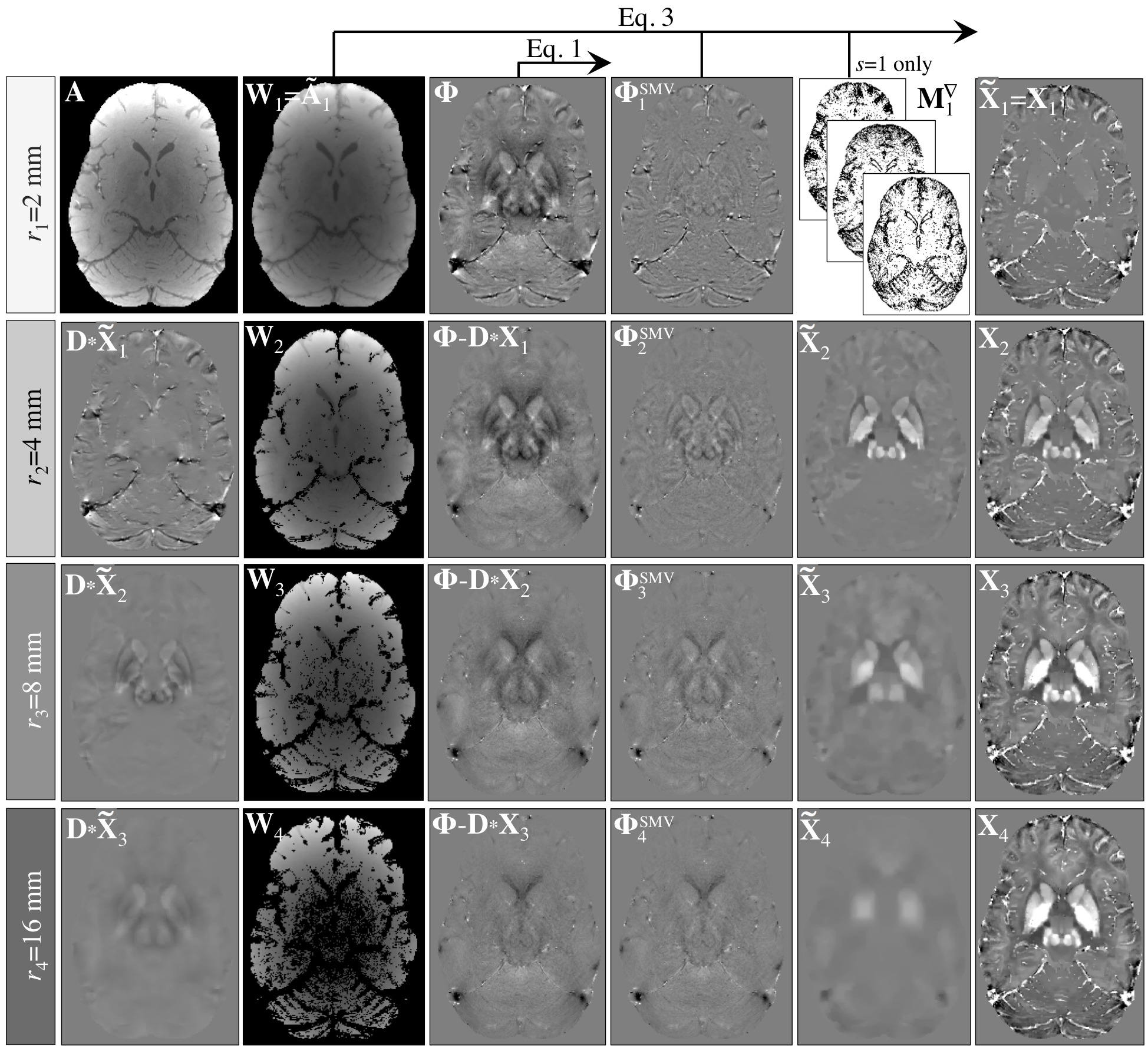
In MSDI (Fig. 1), the susceptibility distribution, $$${\bf{X}}_{s}$$$, is the sum of susceptibility estimates from $$$s$$$ scales, i.e. $$${\bf{X}}_{s}=\left(\chi_{ij}\right)={\operatorname{diag}}\left(\chi_{1}...\chi_{n}\right)=\sum_{s}{\bf{\tilde{X}}}_{s}$$$, each subject to a specific SMV pre-filtering level such that:
$$${\bf{\Phi}}_s^{\tiny{\operatorname{SMV}}}={\bf{\Phi}}_s-{\bf S}_s\ast{\bf{\Phi}}_s$$$, [Eq. 1]
where $$${\bf{\Phi}}_s$$$ and $$${\bf{\Phi}}_s^{\tiny{\operatorname{SMV}}}$$$ represent a phase distribution and its SMV-filtered counterpart, respectively, and $$${\bf{S}}_s$$$ is the SMV kernel with radius, $$$r_s$$$. The algorithm is reinitialised at each scale as follows:
$$${\bf{\Phi}}_s={\bf{\Phi}}-{\bf{S}}_s\ast{\bf{D}}\ast{\bf{X}}_{s-1}$$$, [Eq. 2]
where $$${\bf{\Phi}}$$$ is the initial phase, $$${\bf{D}}$$$ is the dipole kernel and $$${\bf{X}}_{s-1}$$$ is the susceptibility-sum from the previous (finer) scale (starting from a null matrix), which prevents noise amplification and erosion leading to the following subproblem:
$$${\bf\tilde X}_s=\underset{\bf\tilde{X}}{\operatorname{argmin}}\lambda\left\|{\bf{W}}_s\left[\operatorname{exp}\left({i}{\bf\tilde{S}}_s\ast{\bf{D}}\ast{\bf{\tilde{X}}}\right)-\operatorname{exp}\left({i}{\bf{\Phi}}_s^{\tiny{\operatorname{SMV}}}\right)\right]\right\|_2^2+\left\|{\bf{M}}_s^\triangledown\nabla\bf{\tilde{X}}\right\|_1$$$, [Eq. 3]
where $$$\lambda$$$ is the regularisation parameter, $$$\bf{I}$$$ represents the identity matrix, $$${\bf\tilde{S}}_s={\bf{I}}-{\bf{S}}_s$$$ is the SMV-deconvolution kernel, $$$\nabla$$$ is the 3D gradient operator, $$${\bf{M}}_s^\triangledown$$$ is a scale-dependent edge-mask i.e. a dynamic morphological constraint to the regulariser, and $$${\bf{W}}_s$$$ is a scale-specific weighting matrix that adaptively controls for model inconsistencies. Analogous to nMEDI, $$${\bf{W}}_s$$$ was initially set to an estimate of the inverse of the phase-noise distribution, $$${\bf{\tilde{N}}}_s^{-1}$$$, in order to compensate for spatially non-uniform measurement-reliability. The noise distribution can be approximated by the inverse of the signal magnitude, $$${\bf{A}}^{-1}$$$ for $$$\bf{\Phi}$$$, and by $$${\bf{A}}_s^{-1}={\bf{S}}_s\ast{\bf{A}}^{-1}$$$ for the second term of Eq. 1; therefore, the inverse of the composite noise distribution at each scale can be calculated as $$${\bf{\tilde{N}}}_s^{-1}={\bf{\tilde{A}}}_s=\left({\tilde{a}_{s_{ij}}}\right)=\left[{\bf{\hat{A}}}^{-2}+{\bf{\hat{A}}}_s^{-2}\right]$$$, with $$${\bf{\hat{A}}}$$$ and $$${\bf{\hat{A}}}_s$$$ normalised by their respective means over $$$\Omega$$$ – a brain-mask calculated with BET26.
Subsequently at each iteration, $$${\bf{W}}_s$$$ is dynamically downscaled
at locations returning large normalised-consistency residuals, $$${\bf{\hat{R}}}_{s,iter}=\left(\hat{r}_{{s,iter}_{ij}}\right)>f$$$, i.e. MERIT1, which prevents unphysical model departures from
dominating the forward-consistency cost. The algorithm was set to run over four
scales (with SMV-kernel radii, $$$r_s=2,4,8,16\space\operatorname{mm}$$$). On the empirical observation that
large-scale features—i.e. those resulting from Eq. 1 using large SMV kernels—require
large-scale compartmentalisation, we also introduce a scale-wise masking rule that
dynamically prevents cost contributions from the top $$$q\frac{r_s}{r_{2}}$$$th percentile (P) of phase second-differences, $$$\Delta{\bf{\Phi}}^{\prime\prime}$$$7. $$${\bf{W}}_s$$$ can thus be
expressed as:
$$${\bf{W}}_s=\begin{cases}\frac{{\tilde{a}_{s_{ij}}}}{\hat{r}_{{s,iter}_{ij}}}&\forall{\left({i,j}\right):{\hat{r}_{{s,iter}_{ij}}}>f}\\0&\forall{\left({i,j}\right)}:\Delta{{\bf{\phi}}_{ij}}^{\prime\prime}>{\operatorname{P}_{100-q\frac{r_s}{r_{2}}}}\lvert{_{_\Omega}}\space\Delta{\bf{\Phi}}^{\prime\prime}\\{\tilde{a}_{s_{ij}}}&\operatorname{otherwise}\end{cases}$$$, [Eq. 4]
with $$$f=6$$$ (nMEDI’s default) and with initial masking percentile, $$$q=10$$$. In keeping with a previous optimisation, $$${\bf{M}}_s^\triangledown$$$ was set to mask out the location of the top-30% magnitude-gradients8, though only for the smallest SMV-kernel radius (i.e. $$$r_s=2\space\operatorname{mm}$$$) where vascular features are most prominent, i.e. where sharing edges with the magnitude image is a justified prior (Fig. 1).
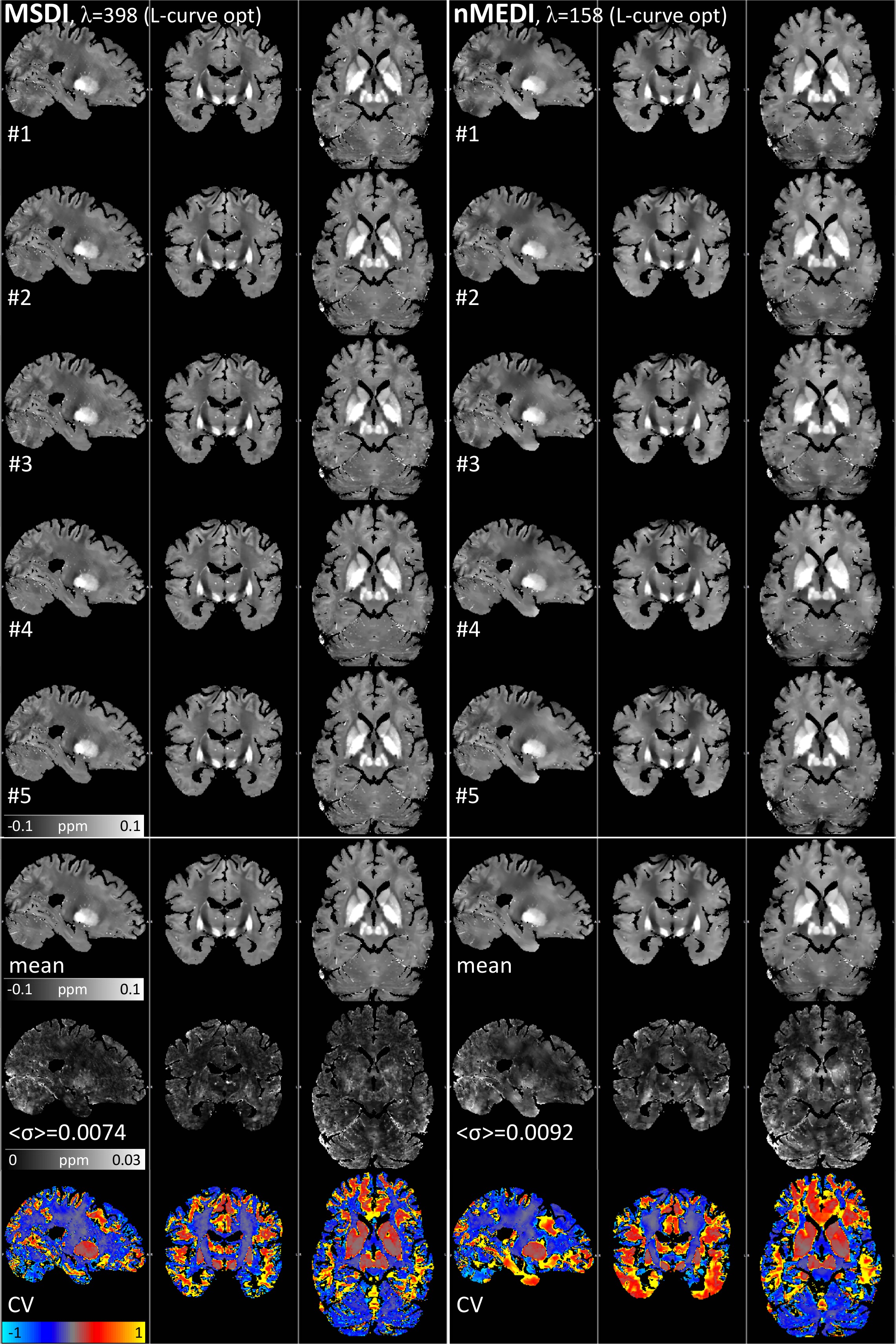
MSDI was compared with state-of-the-art methods in the context of the 2016 QSM Reconstruction Challenge9. We also investigated MSDI-reproducibility in relation to nMEDI through scanning a single subject on five consecutive days with a 2×2-accelerated, spoiled-FLASH sequence, 0.8-mm isotropic voxels, α=12° and eight bipolar echoes ($$$TE_{min}/\space\Delta{TE}/\space{TR}/\space{TA}=2.34\space\operatorname{ms}/2.30\space\operatorname{ms}/25\space\operatorname{ms}/7{\colon}08\space\operatorname{min}$$$) acquired on a Siemens-Trio 3T system with a 32-channel head-coil. Regarding QSM pre-processing, SENSE-based reconstruction was followed by spatial phase unwrapping7, magnitude-weighted least-squares phase fitting with bipolar-readout and transmit-related offset adjustment, and background-phase removal in two steps consisting of Laplacian boundary-value10 and variable-SMV pre-filtering ($$$r_0=25\space\operatorname{mm}$$$)11. All maps were spatially standardised to a study-wise space using an optimised ANTs routine (http://stnava.github.io/ANTs).
Results
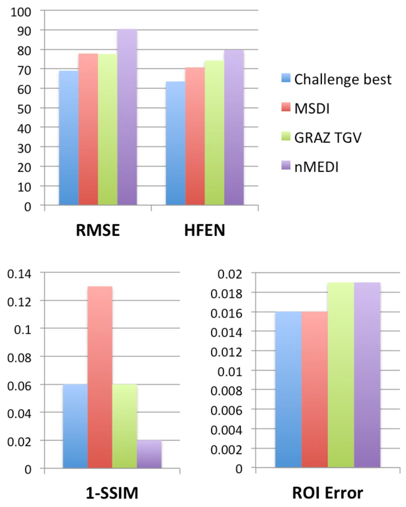
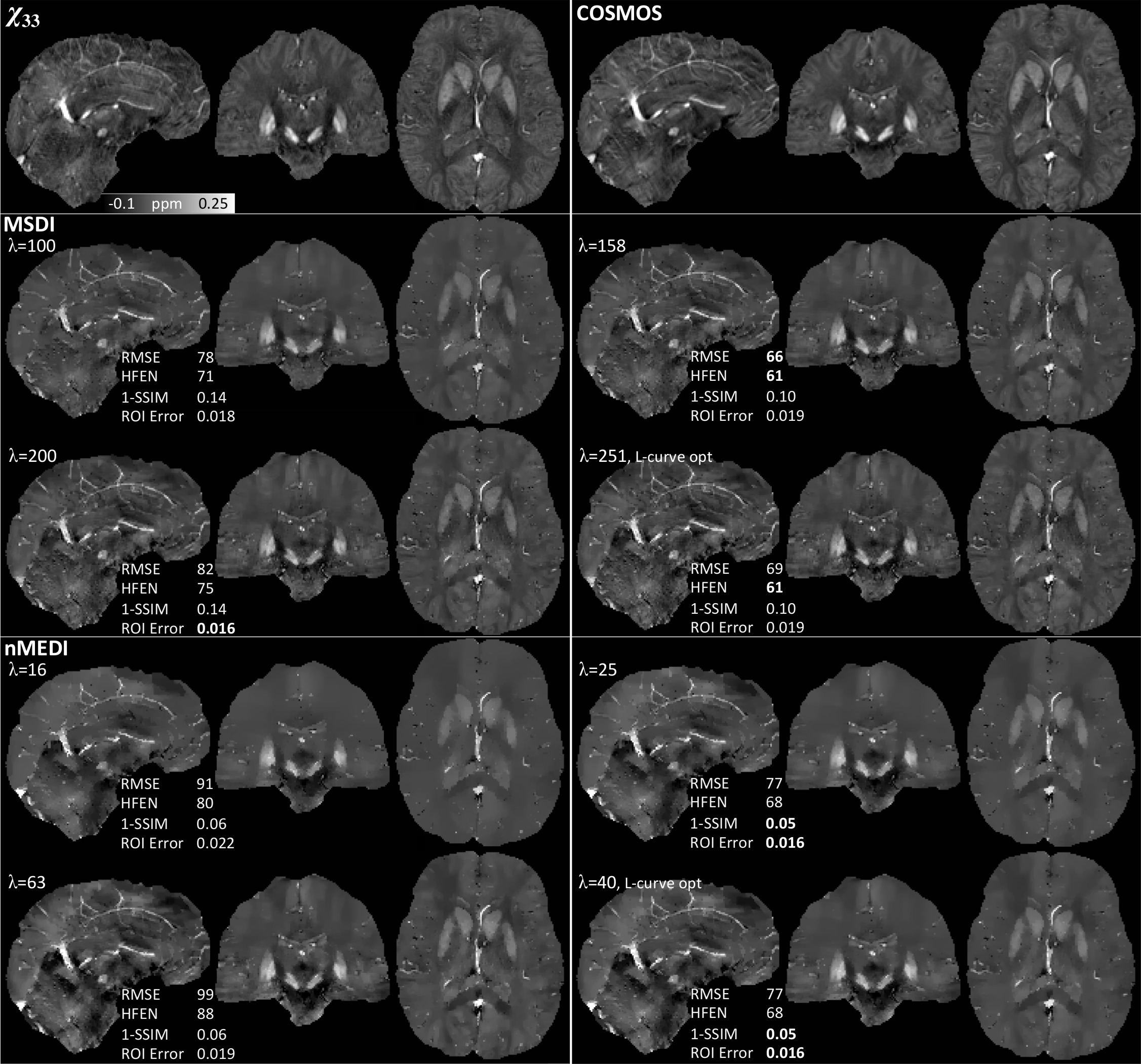
Unlike any other method evaluated in the context of the 2016 QSM Challenge, MSDI ranked in the top-10 for all performance metrics (Fig. 2). As with most other algorithms, slightly different MSDI λs minimised different metrics using the Challenge data (Fig. 3). Interestingly, for an intermediate λ, most scores were further reduced using a COSMOS12 ground-truth (Fig. 3, right column). L-curve analyses13 returned cost-balanced λs that were, as a whole, in a desirable range, though possibly more concordant with COSMOS-based predictions. Qualitatively, MSDI yielded in vivo reconstructions with greater anatomical detail and more uniform appearance than nMEDI; the latter was confirmed by lower test-retest variability across five-repeat measurements (Fig. 4).Discussion & Conclusion
Recent QSM studies proposed the integration of background-removal principles within single-step formulations3,14. However, in their current form they might be vulnerable to artefactual streaking propagation due to insufficient phase-noise/error considerations. We hereby propose a multi-scale approach (MSDI) that enables tighter error control via step-wise SMV deconvolution and dynamic consistency rejection, which in the present study led to robust convergence pathways resulting in accurate and stable reconstructions.Acknowledgements
The Wellcome Centre for Human Neuroimaging is supported by core funding from the Wellcome [203147/Z/16/Z]. FONDECYT 1161448, CONICYT Programa PIA Anillo ACT1416, and Becas de Doctorado Nacional CONICYT, Folio 21150369 (Chile).References
1. Liu T, Wisnieff C, Lou M, et al. Nonlinear formulation of the magnetic field to source relationship for robust quantitative susceptibility mapping. Magn Reson Med 2013;69:467-476.
2. Wang S, Liu T, Chen W, et al. Noise Effects in Various Quantitative Susceptibility Mapping Methods. IEEE Trans Biomed Eng 2013;60:3441-3448.
3. Chatnuntawech I, McDaniel P, Cauley SF, et al. Single-step quantitative susceptibility mapping with variational penalties. NMR Biomed. In press. doi: 10.1002/nbm.3570.
4. Liu T, Liu J, de Rochefort L, et al. Morphology enabled dipole inversion (MEDI) from a single-angle acquisition: comparison with COSMOS in human brain imaging. Magn Reson Med 2011;66:777-783. 5. Liu J, Liu T, de Rochefort L, et al. Morphology enabled dipole inversion for quantitative susceptibility mapping using structural consistency between the magnitude image and the susceptibility map. Neuroimage 2012;59:2560-2568.
6. Smith SM. Fast robust automated brain extraction. Hum Brain Mapp 2002;17:143-155.
7. Abdul-Rahman HS, Gdeisat MA, Burton DR, et al. Fast and robust three-dimensional best path phase unwrapping algorithm. Appl Opt 2007;46:6623-6635.
8. Liu T, Xu W, Spincemaille P, et al. Accuracy of the morphology enabled dipole inversion (MEDI) algorithm for quantitative susceptibility mapping in MRI. IEEE Trans Med Imaging 2012;31:816-824.
9. Langkammer C, Schweser F, Shmueli K, et al. Quantitative susceptibility mapping: Report from the 2016 reconstruction challenge. Magn Reson Med. In press. doi: 10.1002/mrm.26830.
10. Zhou D, Liu T, Spincemaille P, Wang Y. Background field removal by solving the Laplacian boundary value problem. NMR Biomed 2014;27:312-319.
11. Li W, Wu B, Liu C. Quantitative susceptibility mapping of human brain reflects spatial variation in tissue composition. Neuroimage 2011;55:1645-1656.
12. Liu T, Spincemaille P, de Rochefort L, et al. Calculation of susceptibility through multiple orientation sampling (COSMOS): a method for conditioning the inverse problem from measured magnetic field map to susceptibility source image in MRI. Magn Reson Med 2009;61:196-204.
13. Hansen P, O’Leary D. The use of the L-curve in the regularization of discrete ill-posed problems. SIAM J Sci Comput 1993;14:1487-1503.
14. Langkammer C,
Bredies K, Poser BA, et al. Fast quantitative susceptibility mapping using 3D
EPI and total generalized variation. Neuroimage 2015;111:622-630.
Figures