4995
Shading Artifact Suppression using Relaxation Map and Machine Learning-based Region Detection for Quantitative Susceptibility Mapping1Toshiba Corporation, Kawasaki, Japan, 2Toshiba Medical Systems Corporation, Otawara, Japan, 3Toshiba Medical Research Institute, Mayfield Village, OH, United States
Synopsis
We propose a dipole inversion method for improving quantitative susceptibility mapping. In conventional methods, shading artifacts often occur near the longitudinal fissure (LF) region of the estimated susceptibility map. Here, we propose an algorithm for LF region detection and regularized inversion, to reduce the shading artifacts. The LF region is automatically detected using information from the T2* map as well as training datasets via machine learning. The proposed method eliminates shading artifacts near the LF region in the susceptibility maps, while also showing negligible change in regions that do not suffer from shading artifacts, such as the basal ganglia.
Purpose
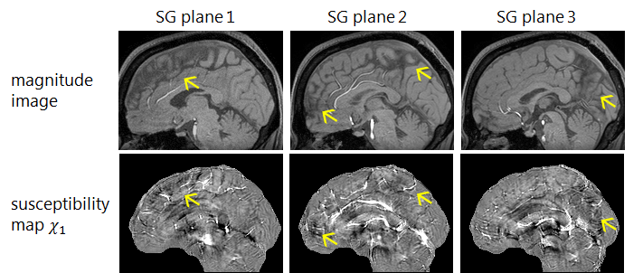
Quantitative Susceptibility Mapping (QSM) estimates tissue magnetic susceptibility that may quantify subtle changes in concentrations of certain biomaterials, such as iron or calcium1-4. In QSM, shading artifacts often occur near regions of tissue-CSF boundaries, including the longitudinal fissure (LF) (Fig.1). The shading artifacts generally have negative value in the susceptibility map (SM), which lead to undesirable results such as the degradation of visibility and accuracy of oxygen extraction fraction calculation5. In this work, we propose a regularized inversion method that reduces the shading artifacts in the LF region of the SM. The LF region is detected by using an automatic segmentation method.
Methods
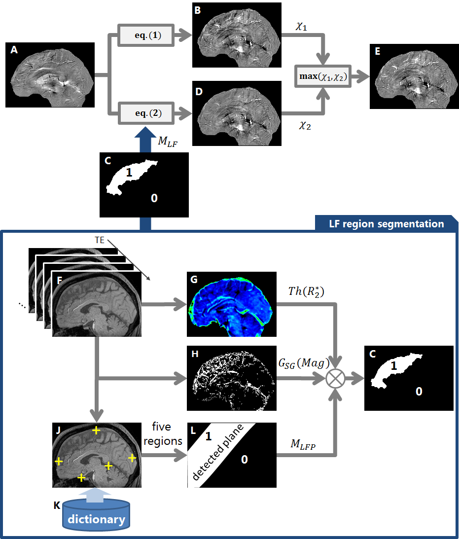
Figure 2 shows the proposed QSM inversion method, which is similar to a formulation reported in previous work6 for the suppression of ventricular CSF inhomogeneity. Our method focuses on the suppression of shading artifacts in the LF region.
QSM Processing
The tissue phase $$$\phi$$$ is estimated using phase unwrapping and background phase removal7,8. Then, two SMs $$$\chi_1$$$ and $$$\chi_2$$$ are generated using two different inversion algorithms from the $$$\phi$$$. The first SM is estimated using eq.(1):
$$\chi_1={\rm{argmin}}_{\chi}\lVert d\chi-\phi\rVert_2+\lambda_1\lVert M_RG\chi\rVert_1,\cdots(1)$$
with $$$d$$$ the dipole kernel, $$$G$$$ the the 3D gradient operator, $$$\lambda_1$$$ the coefficient for the edge-weighted local susceptibility consistency term. $$$M_R$$$ is the the binary edge mask, which is derived from the R2* map. Let $$$\chi_1$$$ be the SM estimate from the conventional method. The second SM is estimated using eq.(2), which adds an L2 artifact suppression term to eq.(1):$$\chi_2={\rm{argmin}}_{\chi}\lVert d\chi-\phi\rVert _2+\lambda_1\rVert M_RG\chi \rVert_1+\lambda_2\rVert M_{LF} (\chi-\bar{\chi})\rVert_2,\cdots(2)$$
with $$$\lambda_2$$$ the coefficient for the artifact suppression term, $$$\bar{\chi}$$$ the mean susceptibility value in LF region (as masked by $$$M_{LF}$$$). $$$M_{LF}$$$ is derived from the magnitude image, R2* map and a machine learning technique:
$$M_{LF}=Th(R_2^*)\cdot G_{SG}(Mag)\cdot M_{LFP},\cdots(3)$$
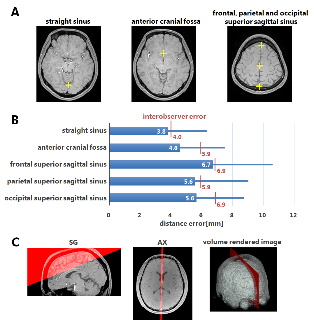
where $$$Th(R_2^*)$$$ is the thresholding $$$R_2^*:Th(R_2^*)=10<R_2^*<40[1/s]$$$ to detected the WM/GM regions, $$$G_{SG}(Mag)$$$ is the edge operator in the sagittal direction of the magnitude image to detect the shading artifact, and $$$M_{LFP}$$$ is the estimated LF plane binary mask. A machine learning-based region detection technique using random forest9 is applied to the magnitude images and the positions of five anatomical regions in the brain are detected (Fig.3A). The LF plane mask $$$M_{LFP}$$$ is computed by using liner regression from these five regions. Using $$$M_{LFP}$$$, it is possible to reduce the masking influence on other regions, e.g. the basal ganglia region and the optic radiations. The final SM $$$\chi$$$ is generated by choosing the larger value of the intermediate SMs for each voxel in order to mitigate the shading artifact.
Data acquisition
Datasets for detection of the LF region: 75 T2*-weighted images were used by the machine learning algorithm.
Datasets for QSM evaluation: five datasets were acquired from five healthy volunteers on a 3T MRI scanner using a 3D gradient echo with the following parameters: $$$ \rm{TE1/\Delta TE/numEchos/TR=5/5/5/29,FA=15,Resolution=1x1x1mm,FOV=256x256x150mm}$$$.
Evaluation
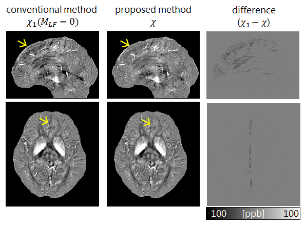
Two readers independently detected the positions of the five brain regions. These measurements served as the reference for assessing the performance of the region detection algorithm. The distance between the estimated coordinates and the two human readers were measured for each region. Errors were computed separately using the leave-one-out cross-validation method and compared to interobserver errors. The proposed inversion method was evaluated based on its ability to eliminate artifacts near the LF region compared to $$$\chi_1$$$, which is equivalent to the proposed method when $$$M_{LF}=0$$$. For quantitative evaluation, susceptibility was measured for each ROI in the brain.
Results and Discussion
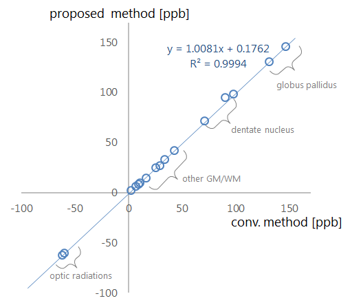
The proposed automatic region detection algorithm detected all five anatomical regions in all 75 datasets. The average difference of the spatial position was 5.3 mm, which is lower than interobserver errors (Fig.3B). The LF plane is also detected from the anatomical regions (Fig.3C). The proposed inversion algorithm eliminates shading artifacts near the LF region compared to the conventional (Fig.4). In non-LF regions, a strong agreement and correlation of susceptibility estimates is observed between the proposed method and the conventional method, suggesting that the proposed method does not significantly alter magnetic susceptibility estimates outside of the LF region (Fig.5). The LF region originally has positive susceptibility10 since voxels in the LF region are in partial volume region of the GM and CSF. Therefore the proposed method leads to more accurate estimates of susceptibility in the LF region by suppressing the negatively-valued shading artifacts.
Conclusion
We have proposed a method to remove shading artifacts in the LF region of SMs, by using additional information from the relaxation map and machine learning-based region detection. The proposed method may also be applied to regions such as the cerebral cortex to improve the estimation of SMs.Acknowledgements
The authors would like to thank Dr. Fushimi (Kyoto University Graduate School of Medicine) for his assistance with the provision of data.References
[1] Haacke EM et. al., Magn Reson Imaging 23(1):1-25
[2] de Rochefort L et. al., Magn Reson Med 60(4):1003-9
[3] Shmueli K et. al., Magn Reson Med 62(6):1510-22
[4] Wang Y et. al., Magn Reson Med 73(4):82-101
[5] Kudo K et. al., J Cereb Blood Flow Metab 36(8):1424-33
[6] Liu Z et. al., Magn Reson Med. doi:10.1002/mrm.26946
[7] Schweser F et. al., NeuroImage. 54(4):2789-807
[8] Shiodera T et. al., Proc Intl Soc Mag Reson Med 24 (2016):1559
[9] Geurts P et. al., Machine Learning 63:3-42
[10] Langkammer C et. al, NeuroImage 62(2012) 1593-99
Figures