4986
True Phase Quantitative Susceptibility Mapping Using Continuous Single Point Imaging: A Feasibility Study1Radiology, University of California San Diego, San Diego, CA, United States, 2Radiology Service, VA San Diego Healthcare System, San Diego, CA, United States
Synopsis
Quantitative susceptibility mapping (QSM) has recently been in the limelight as a novel contrast mechanism to provide quantification of apparent magnetic susceptibility based on phase information in MR images. In this study, we explore feasibility of single point imaging (SPI) for QSM. SPI, also known as constant time encoding or pure phase encoding, provides true phase information not affected by phase evolution during readout, which is beneficial for accurate QSM. We propose a new and efficient SPI acquisition scheme for QSM, termed Continuous SPI, where SPI images are continuously obtained with extremely high temporal resolution in a single scan.
Introduction
Quantitative susceptibility mapping (QSM) has recently surfaced as a powerful biomarker for iron deposition, calcification, oxygenation, and demyelination. QSM utilizes phase evolution over multiple different echo times (TE), and hence it is crucial to acquire accurate phase information. In this study, we explore feasibility of a new imaging technique for QSM utilizing single point imaging (SPI), also known as constant time encoding, where an entire k-space is encoded at a same TE (i.e., zero readout duration), which captures a snapshot of true phase. The conventional SPI is further modified to enable continuous imaging with extremely high temporal resolution (echo spacing=16µs), which we termed Continuous SPI.Methods
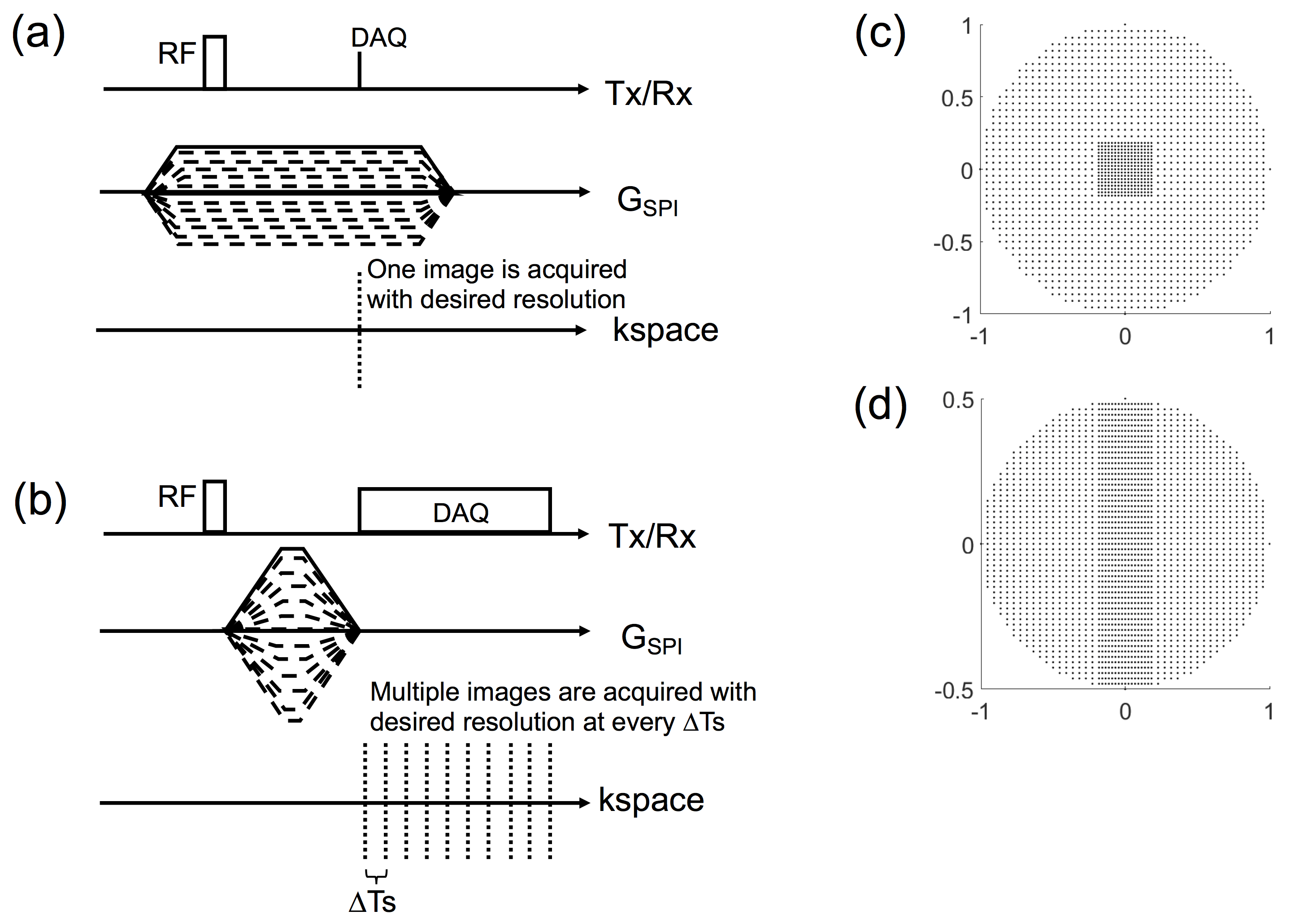
Figure 1-a shows a pulse sequence diagram (PSD) for conventional SPI, where a short hard pulse and a plateau of gradient are typically used for imaging. 3D SPI is performed by linearly scaling (e.g., from -1x to 1x) the maximum phase encoding gradients in three gradient axes in each TR. Unfortunately, this scheme is very time-intensive and hence not suitable for scenarios that typically require multiple acquisitions, such as quantitative imaging. Figure 1-b shows the PSD for the proposed Continuous SPI, where gradients are rapidly ramped up after RF excitation to remove unwanted slice selectivity artifacts1 and then switched off once desired resolution is achieved. After switching off the gradients, k-space data are continuously sampled at a fixed k-space location with a temporal resolution determined by sampling interval, ∆Ts (=1/sampling BW). Note that the maximum phase encoding gradient must be designed to have the desired area= 2πN/(γFOV) (γ: gyromagnetic ratio, FOV: field of view, N: matrix size) to achieve desired resolution. Figure 1-c and d show an example of 3D phase encoding steps used for the proposed Continuous SPI. Note that parallel imaging with auto-calibration is utilized to accelerate SPI imaging.
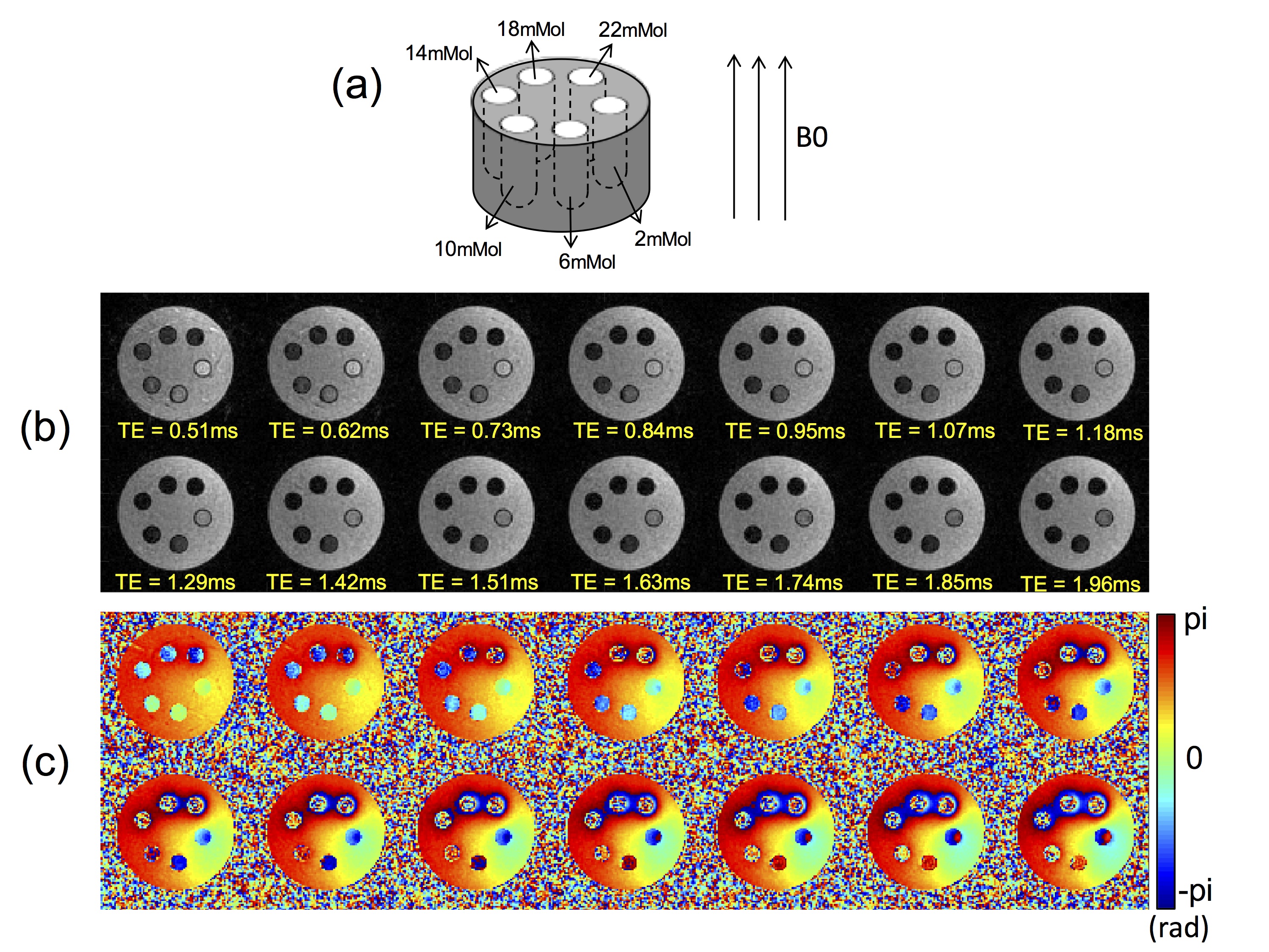
To evaluate the proposed method, a phantom comprised of six tubes surrounded by agarose gel (1% by weight) was prepared, where each tube was filled with 2mL of Feridex I.V. solution (Berlex Laboratories, Wayne, New Jersey, USA), with six different iron concentrations ([Fe]=2, 6, 10, 14, 18, and 22 mMol) as shown in Figure 2-a. The phantom was imaged at 3T (MR750, GE Healthcare, Waukesha, WI, USA) using an 8-ch T/R knee coil, with the longitudinal direction of the tubes placed parallel to the B0 field. Continuous SPI was performed using the following imaging parameters: RF=24µs hard pulse, FA=6°, slewrate=200mT/m/msec, voxelsize=1x1x2mm, FOV=89x89x110mm, acceleration factor for parallel imaging=2x2x1, a matrix size for auto-calibration=17x17x55, ∆Ts=16µs, TE=506, 522, …, 2010µs (total 95 TEs), TR=4.5ms, scantime=5min16sec. All 95 images were reconstructed utilizing GRAPPA2. For comparison, a 3D-Cones sequence was used for imaging with FOV/voxelsize matched to SPI with the following imaging parameters: RF=628µs SLR pulse with minimum phase, FA=15°, TE=32, 132, 232, 332, 432, and 532µs (acquired with 6 scans), TR=8ms, scantime=7min. In the proposed Continuous SPI, 14 out of total 95 images were used for QSM analysis based on Morphology Enabled Dipole Inversion (MEDI)3.
Results
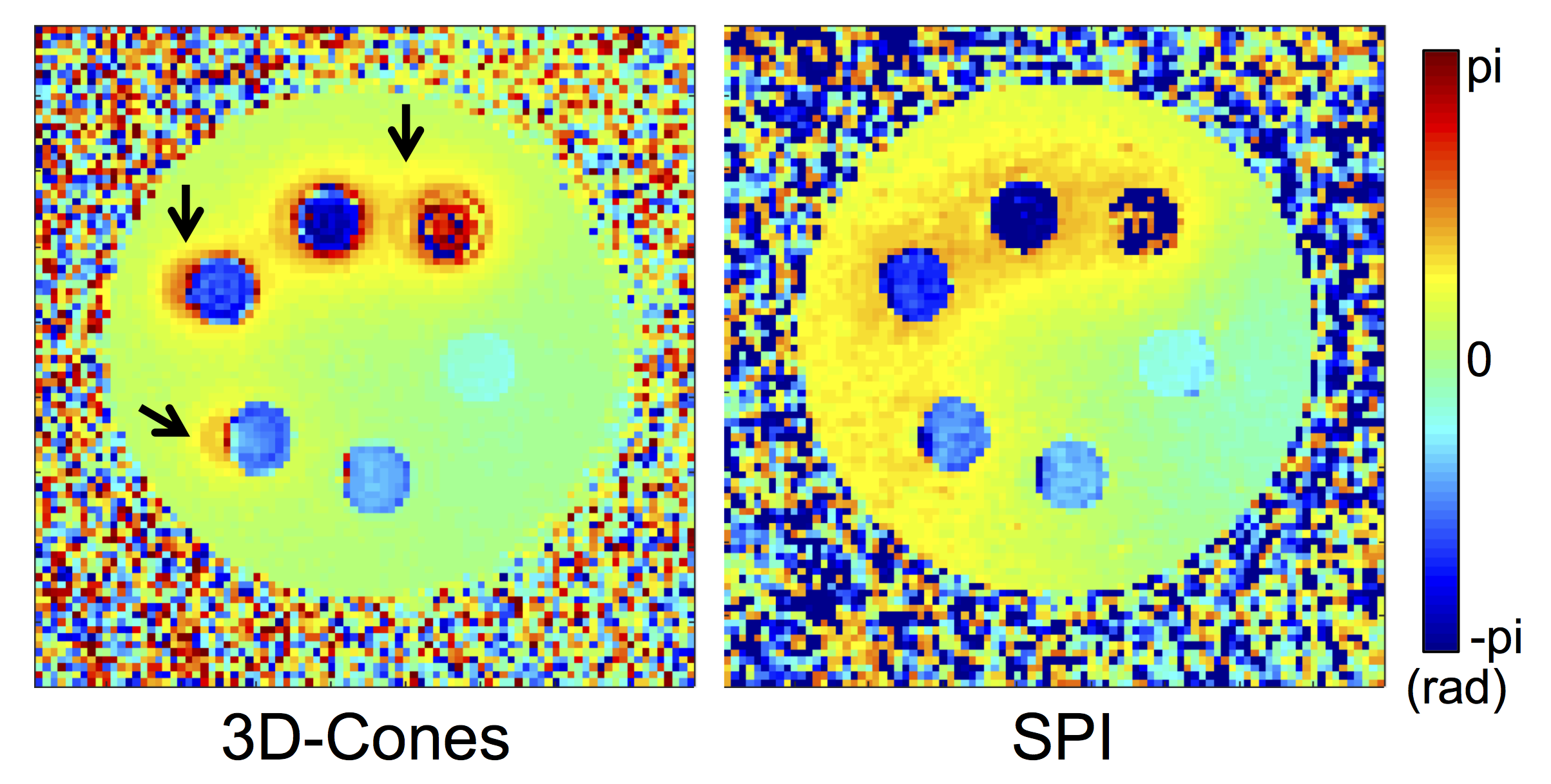
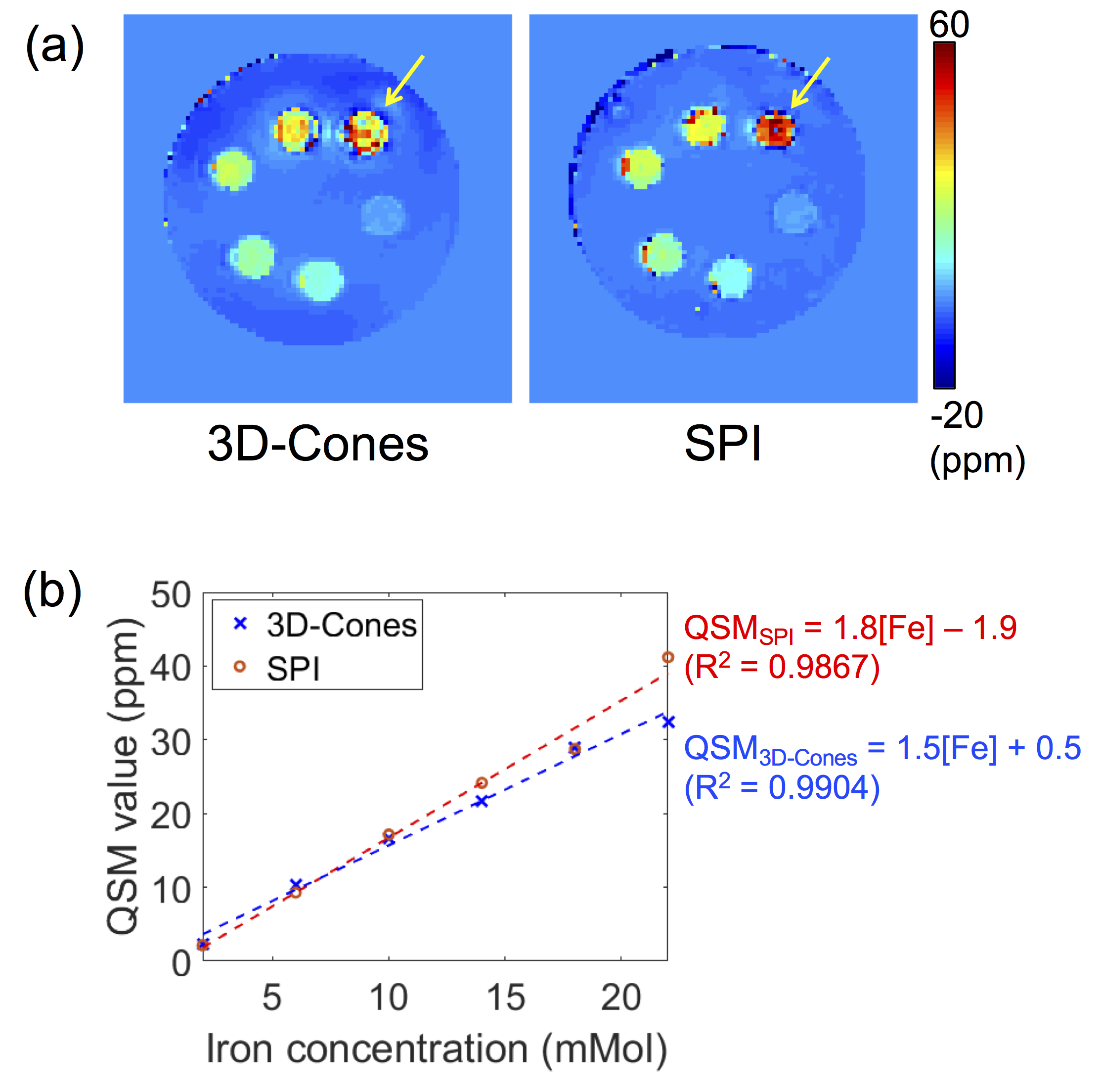
Figures 2-b and c show magnitude and phase images at 14 different TEs in Continuous SPI, used for QSM analysis. Figure 3 shows phase maps in the same location acquired by 3D-Cones (TE=532µs) or Continuous SPI (TE=538µs). The 3D-Cones phase map shows strong ringing near tubes with high iron concentrations (black arrows) due to off-resonance effects from frequency encoding, while SPI (pure phase encoding) does not exhibit such artifactual ringing. Figure 4-a shows a result of QSM using 3D-Cones or SPI. As seen, 3D-Cones and SPI showed overall similar values except at the highest iron concentration (yellow arrows). Figure 4-b shows mean QSM values in each tube, where SPI shows very strong linearity in the first 4 tubes (with [Fe]=2, 6, 10, 14mMol), while QSM values estimated for 2 tubes with high iron concentrations may have shown variability due to low SNR.Discussion and Conclusion
In this study, we explored the feasibility of QSM acquired using Continuous SPI, which is a robust and efficient technique that provides true phase information. The proposed method has many potential clinical applications, including patients with metallic implants4 or hemophilia. Moreover, Continuous SPI is more robust to motion since images are acquired in a single scan. One inherent limitation of SPI is that the minimum TE depends on desired resolution, but this can be overcome by incorporating more advanced techniques5,6. In future works, we will evaluate the efficacy of the proposed imaging scheme with more extensive phantom and in vivo experiments.Acknowledgements
The authors acknowledge grant support from NIH (1R01 AR062581, 1R01 AR068987, and 1R01 NS092650), VA Clinical Science Research & Development Service (Merit Award 1I01CX001388), and GE Healthcare.References
1. Jang H, Wiens CN, McMillan AB. Ramped hybrid encoding for improved ultrashort echo time imaging. Magnetic Resonance in Medicine. 2016;76(3):814–825.
2. Griswold MA, Jakob PM, Heidemann RM, Nittka M, Jellus V, Wang J, Kiefer B, Haase A. Generalized autocalibrating partially parallel acquisitions (GRAPPA). Magnetic resonance in medicine. 2002;47(6):1202–10.
3. De Rochefort L, Liu T, Kressler B, Liu J, Spincemaille P, Lebon V, Wu J, Wang Y. Quantitative susceptibility map reconstruction from MR phase data using bayesian regularization: Validation and application to brain imaging. Magnetic Resonance in Medicine. 2010;63(1):194-206.
4. Wiens CN, Artz NS, Jang H, McMillan AB, Koch KM, Reeder SB. Fully phase-encoded MRI near metallic implants using ultrashort echo times and broadband excitation. Magnetic Resonance in Medicine. 2017;In Press.
5. Jang H, Subramanian S, Devasahayam N, Saito K, Matsumoto S, Krishna MC, McMillan AB. Single Acquisition Quantitative Single-Point Electron Paramagnetic Resonance Imaging. Magnetic Resonance in Medicine. 2013;70(4):1173–1181.
6. Kaffanke JB, Romanzetti S, Dierkes T, Leach MO, Balcom BJ, Jon Shah N. Multi-Frame SPRITE: A method for resolution enhancement of multiple-point SPRITE data. Journal of Magnetic Resonance. 2013;230C:111–116.
Figures