4902
Motion Correction for 3D+time Cardiac MRI Perfusion Images1Electrical and Computer Engineering, University of Utah, Salt lake City, UT, United States, 2UCAIR, University of Utah, Salt Lake city, UT, United States
Synopsis
A motion correction technique for 3D dynamic cardiac perfusion MRI using rigid and non-rigid image registrations to improve quantification of cardiac perfusion is presented. This method is unique because it employs a 3D image registration which not only resolves in plane motion but also resolves the out of plane motion for all slices in a 3D volume. This method also ensures smooth registration between all time frames of the data giving a more accurate analysis of the flow values.
Introduction
Dynamic contrast-enhanced magnetic resonance imaging can be useful to quantify myocardial ischemia. However, patient respiratory motion can
affect the accuracy of subsequent analyses making the quantification poor. Motion correction techniques are always an extra
challenge for dynamic contrast enhanced data since the intensity changes rapidly over time. In case of myocardial perfusion, there is
respiratory motion, cardiac motion and the patient can move. All these things combined make the problem difficult to solve.
Most cardiac perfusion sequences acquire multiple 2D slices. Several 3D methods have been published 6,7 but they have employed breath-holding and no registration in the post-processing steps for quantification. Here, we present a new motion correction technique which uses rigid and nonrigid registration methods for removing motion from 3D time series data. The 3D acquisition has the advantage that out-of-plane motion can be registered (though not out-of-slab motion).
Methods
In our method, the problem of contrast change is dealt by creating model based image volumes.3 Fig 1 shows the general idea of using a model-based method to create individual reference image for each time frame. These model images are reference volumes for the rigid registration which uses a normalized cross correlation metric for finding rigid shifts. Next, we use a non-rigid registration method which is a greedy diffeomorphic algorithm. These “greedy” algorithms iteratively apply gradient updates to a single deformation field, rather than update a full time-dependent flow each iteration. Algorithms in this class include the original diffeomorphic image registration algorithm of Christensen et al. 1 and the diffeomorphic demon’s algorithm of Vercauteren et al.4
In our method,$$$I_{0}$$$ is the 3D image volume taken at time frame T and $$$I_{1}$$$ is the 3D image volume taken at T+1. Also, the deformation field is initially defined as identity and changes as the algorithm progresses with the number of iterations. Fig 2 is a deformed 3D field at time T which is used to interpolate the input image.
This greedy non-rigid image registration technique uses the cost function1,2 given below
$$E(\phi) = \parallel I_{0}\circ\phi-I_{1}\parallel_{L_{2}}^{2}.$$
where $$$\phi$$$ is the deformation field which changes for every iteration till the cost function converges.
Formally, the greedy algorithm can be interpreted as
gradient descent of the manifold of diffeomorphisms:
$$ \frac{\text{d}\phi^{-1}}{\text{d}t} = K\triangledown(I_{0}\circ\phi^{-1})(I_{0}\circ\phi^{-1}-I_{1}).$$
Here $$$K$$$ is a linear differential kernel
operator defined as
$$$
K = (1-\alpha\triangle)^{-S} $$$, $$$\triangle$$$ is a Laplacian operator
and $$$K$$$ in general acts as a low pass filter and suppresses high frequency
components in the image matching gradient. For best deformations, S should be 2<S<5.
The algorithm was tested for five 3D datasets. All the acquired MRI dataset have matrix size 144x144x8 and were initially registered rigidly with
the model images using a normalized cross correlation metric. Then a greedy
diffeomorphic registration is performed with the following parameters α=30, S=2. With 100 iterations for gradient descent, our model takes ~12 minutes to register the entire 3D data +100 time frames in MATLAB 2017a ,The MathWorks, Inc., Natick, Massachusetts, United States.
Results
Fig 2 is the deformation field for one slice and shows significant motion at distinct positions in the deformation field. The rigid shifts do not resolve the overall motion and non-rigid registration reduced motion around the chest wall which is the major peak in Fig 2. Fig 3 shows the warping of the slice in all directions. Fig 4 is a line profile through a slice before and after registration for all time frames. We selected 2 regions between the epicardium and endocardium to show the variation of SI vs time frame curve before and after registration (Fig 5). Our purposed method can improve further quantification of myocardial perfusion by providing motion reduced images.Discussion
This method was found to be effective when there was considerable motion. It was observed the sudden motion of the myocardium was resolved with the help of rigid shifts, and the overall motion was reduced using the greedy diffeomorphic registration. Furthermore, we see that this method deals with out of plane motion as shown in Fig 2, the peaks and troughs show how much the out of plane motion can affect the 3D cardiac MRI data.Conclusion
We presented a motion correction technique for 3D contrast enhanced cardiac MRI perfusion. We first did a rigid registration and then followed by a non-rigid registration for our data. After performing this type of motion correction, the processing for quantification of myocardial perfusion is likely to be more accurate and give better analysis of flow values.Acknowledgements
No acknowledgement found.References
- Christensen, G.E., Rabbitt, R.D., Miller, M.I.: Deformable templates using large deformation kinematics. IEEE Transactions on Image Processing 5(10), 1435–1447 (1996).
- Beg, M., Miller, M., Trouv´e, A., Younes, L.: Computing large deformation metric mappings via geodesic flows of diffeomorphisms. International Journal of Computer Vision 61(2), 139–157 (2005)
- G. Adluru, E. V. R. DiBella, and M. C. Schabel. Model-based registration for dynamic cardiac perfusion mri. Journal of Magnetic Resonance Imaging, 24(5):1062– 1070, 2006.
- Vercauteren, T., Pennec, X., Perchant, A., Ayache, N.: Diffeomorphic demons: Efficient non-parametric image registration. NeuroImage 45(1), S61–S72 (2009).
- D. Likhite, G. Adluru, E. DiBella, "Deformable and rigid model-based image registration for quantitative cardiac perfusion" in Statistical Atlases and Computational Models of the Heart-Imaging and Modelling Challenges, New York, NY, USA:Springer, pp. 41-50, 2015.
- Wissmann, L., Gotschy, A., Santelli, C. Analysis of spatiotemporal fidelity in quantitative 3D first-pass perfusion cardiovascular magnetic resonance. J Cardiovasc Magn Reson. 2017.
- Wissmann, L., Niemann, M., Gotschy, A., Manka, R. Quantitative
three-dimensional myocardial perfusion cardiovascular magnetic
resonance with accurate two-dimensional arterial input function
assessment. J
Cardiovasc Magn Reson. 2015.
Figures
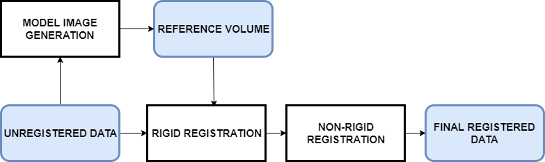
Fig 1:
Registration Model
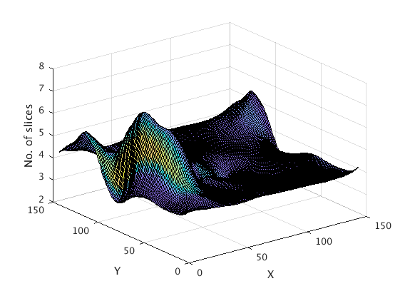
Fig 2 :
Deformation field grid for a single slice at a time frame T showing out of plane motion in the Z direction. The peaks and troughs show how much the out of plane motion can affect the data. Peaks around the left corner and the trough around the center show significant out of plane motion of the chest wall and the myocardium.
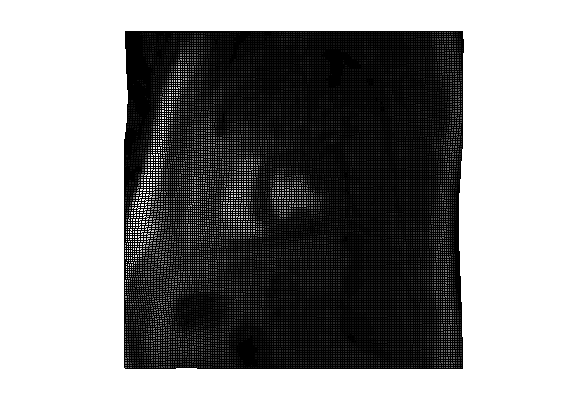
Fig 3 :
Top view of the deformation field grid showing the interpolation between a single slice and the deformed field grid at time frame T. It shows the warping of a single slice along the deformed grid.
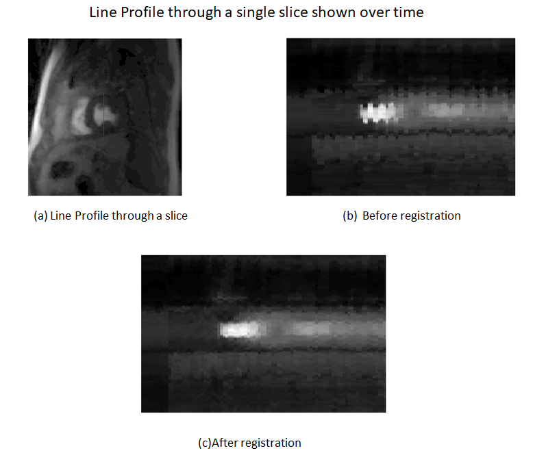
Fig 4:
Line profile for registered data is smooth with no motion and for the unregistered data motion is clearly seen.
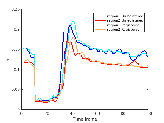
Fig 5 :
Plot of SI vs time frame curve of 2 regions in the myocardium of a single slice for registered and unregistered data. The first 10 frames represent proton density signal followed by 20 baseline frames and then the contrast agent uptake is observed after time frame 30. There is a significant difference for both regions SI curves for the registered and unregistered data. During contrast uptake there is considerable disturbance in the unregistered data in comparison to the registered data. As well, towards the very end of the time series the curve is not smooth for the unregistered data.