4809
Magnetic Susceptibility Mapping Reveals Altered Vein Oxygenation in Patients with Brain Arteriovenous Malformations: A Preliminary Study1Medical Physics and Biomedical Engineering, University College London, London, United Kingdom, 2The Gamma Knife Centre at Queen Square, National Hospital for Neurology and Neurosurgery, London, United Kingdom, 3Department of Neurosurgery, National Hospital for Neurology and Neurosurgery, London, United Kingdom, 4The Lysholm Department of Neuroradiology, National Hospital for Neurology and Neurosurgery, London, United Kingdom, 5Academic Neuroradiological Unit, Department of Brain Repair and Rehabilitation, University College London, London, United Kingdom, 6Academic Neuroradiological Unit, Department of Brain Repair and Rehabilitation, Institute of Neurology, University College London, London, United Kingdom, 7Leonard Wolfson Experimental Neurology Centre, Institute of Neurology, University College London, London, United Kingdom
Synopsis
Arteriovenous malformations (AVMs) are vascular anomalies characterised by arteriovenous shunting with the lack of a capillary bed. Since the veins that drain an AVM contain arterialised blood, they would be expected to have a higher venous oxygen saturation (SvO2) than normal veins. Due to the paramagnetic properties of deoxyhaemoglobin, SvO2 can be calculated using magnetic susceptibility mapping (SM). Here, we calculated SM-based SvO2 in five patients with a brain AVM. We found higher SvO2 in the AVM draining veins compared to normal veins, showing that SM might be a valuable tool to study AVM physiology.
Introduction
Arteriovenous malformations (AVMs) are vascular anomalies characterised by arteriovenous shunting through a network of coiled and tortuous vessels, with the lack of a capillary bed. AVMs are characterised by abnormal blood flow and by the presence of more oxygenated, higher pressure blood in the draining veins1,2.
Previous studies3-5 have shown that magnetic susceptibility mapping (SM) can be used to calculate values of venous oxygen saturation (SvO2) due to the paramagnetic properties of deoxyhaemoglobin:
$$SvO_2[\%]=100-\frac{{\Delta}\chi_{vein-water}-{\Delta}\chi_{oxy-water}Hct}{{\Delta}\chi_{do}Hct}\qquad[1]$$
where $$${\Delta}\chi_{vein-water}$$$ is the magnetic susceptibility ($$$\chi$$$) shift between venous blood and water measured using SM, Hct the haematocrit, $$${\Delta}\chi_{do}$$$ the $$$\chi$$$ shift per unit Hct between fully oxygenated and fully deoxygenated erythrocytes, and $$${\Delta}\chi_{oxy-water}$$$ the $$$\chi$$$ shift between oxygenated blood cells and water.
In a previous study6, we showed that SM could detect the presence of a brain AVM due to the malformation’s increased venous density. Here, we tested whether SM can detect increased SvO2 in a brain AVM’s draining veins based on images of five patients with a brain AVM, before treatment with gamma-knife radiosurgery.
Methods
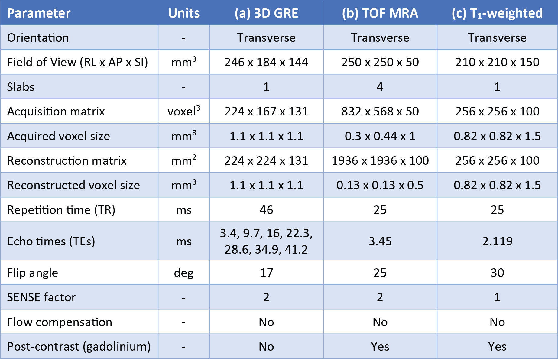
Five patients were scanned with a Philips Achieva 3T system (Best, NL) using a 32-channel head coil. The protocol included a whole-brain 3D multi-echo gradient-echo (GRE) scan for SM (Table 1a); a post-contrast time-of-flight magnetic resonance angiography (MRA) scan for high-resolution imaging of the brain area containing the AVM (Table 1b); and a whole-brain post-contrast T1-weighted scan (Table 1c).
For each patient, a brain mask was created using ITK-Snap7 and the last-echo magnitude image of the GRE data set. SM was performed based on the GRE images, using a previously described processing pipeline6, which included multi-echo fitting of the complex MRI signal8, phase unwrapping using SHARP9, background field removal using PDF10 followed by a 3-voxel erosion of the brain volume10, and local field-to-susceptibility inversion using STAR-QSM11.
Since $$$\chi$$$ measurements are inherently relative, they must be referenced to a standard tissue region to enable the comparison of SvO2 across subjects. Here, $$$\chi$$$ was referenced to the posterior limb of the internal capsule12 (IC-posterior). IC-posterior was delineated based on the Eve susceptibility atlas13, which was coregistered to each patient’s skull-stripped fourth-echo magnitude image (TEEve/TE4 = 22.3/24 ms) using NiftyReg14,15.
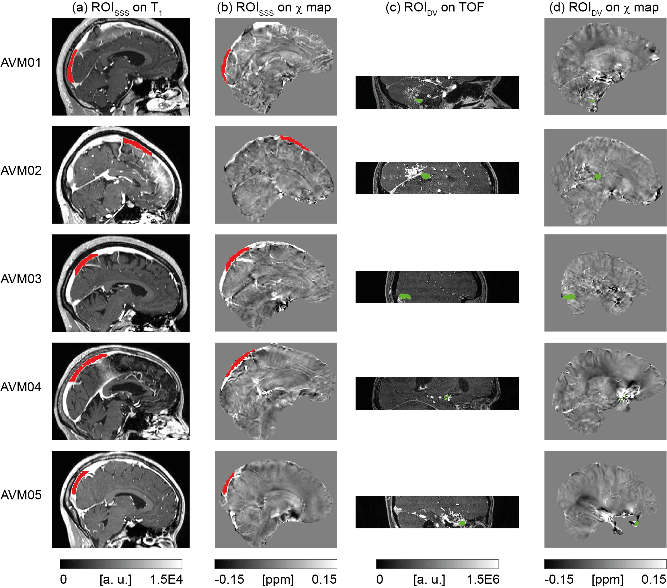
For each patient, two ROIs were drawn using ITK-SNAP7: one (ROIDV) in a vein draining the AVM, the other (ROISSS) in a region of the superior sagittal sinus (SSS) that did not drain blood from the AVM, and, therefore, could be regarded as healthy. ROIDV was drawn on the TOF image and had a different size for each patient due to the variable anatomy of the AVMs. As, depending on the location of the AVM, the TOF image did not always include the SSS, ROISSS was drawn on the T1-weighted image. ROISSS had a similar size across patients but was drawn on different locations of the SSS, to ensure the exclusion of regions draining blood from the AVM. Both ROIDV and ROISSS were then coregistered to the $$$\chi$$$ map using NiftyReg14,15.
For each patient, SvO2 was measured in each voxel of both ROIDV and ROISSS using Equation [1] and $$${\Delta}\chi_{do}=0.27\cdot4\pi$$$ ppm16, $$${\Delta}\chi_{oxy-water}=-0.03\cdot4\pi$$$ ppm4 and individual measures of Hct (40.3±3.08%) taken within three weeks before the MRI scan. For each patient, the mean and standard error of the mean (SEM) of SvO2 were calculated in each ROI, along with the average difference of SvO2 between ROIs. Moreover, the means and SEMs of SvO2 were calculated across patients.
Results and Discussion
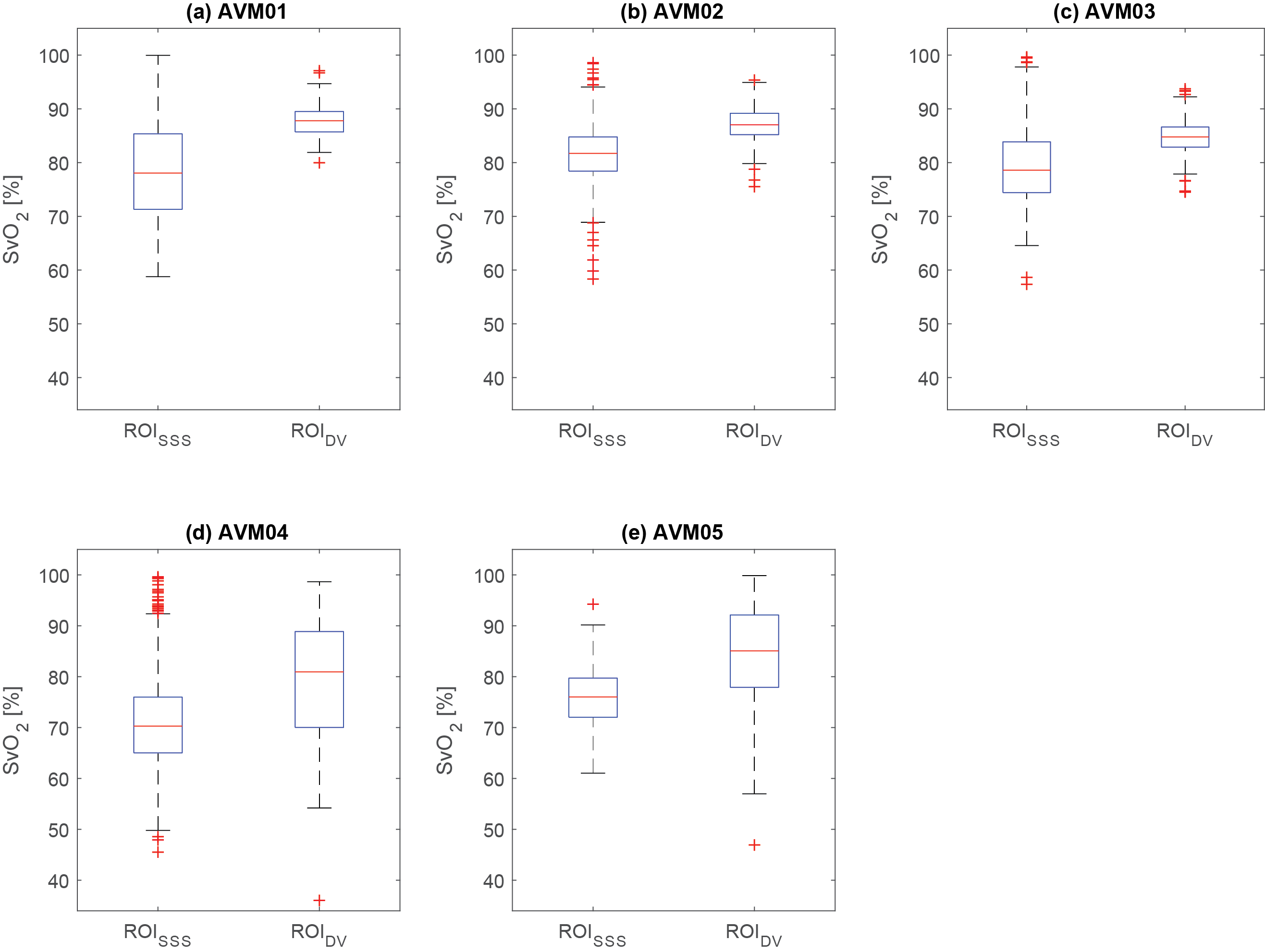
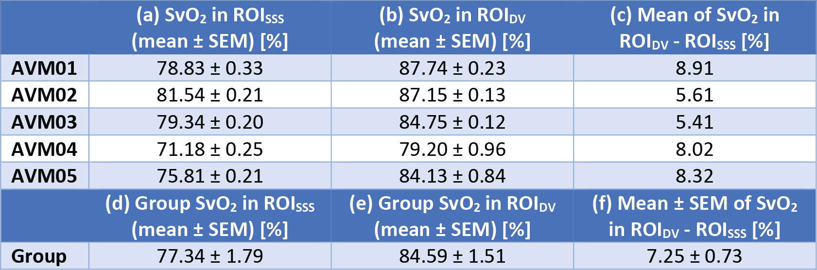
For each patient, Figure 1, Figure 2 and Table 2 respectively show the location of ROISSS and ROIDV, the distribution of SvO2, and the mean±SEM of SvO2. The average SvO2 was always larger in ROIDV than in ROISSS (Figures 2a-e and Table 2a-c).
In ROISSS of all patients and ROIDV of patients AVM01-03, the SEM of SvO2 had consistent values (Table 2a-b and Figure 2). However, in ROIDV of patients AVM04-05, the SEM of SvO2 was larger (Table 2b and Figure 2d-e). In AVM04, this might be due to the proximity of ROIDV to a region containing paramagnetic by-products of a previous haemorrhage; in AVM05 it is likely to be due to the proximity of ROIDV to the edge of the brain volume.
Conclusions and Future Work
We have shown that SM can be used to detect SvO2 alterations in brain AVMs. We report higher SvO2 in the veins draining an AVM than in healthy veins. This information has potential implications for the study of AVM pathophysiology and the clinical evaluation of patients with AVMs using SM. Future work will involve calculating SvO2 in a larger cohort of patients.Acknowledgements
DLT is supported by the UCL Leonard Wolfson Experimental Neurology Centre (PR/ylr/18575).References
- Dillon WP. Cryptic vascular malformations: Controversies in terminology, diagnosis, pathophysiology, and treatment. Am J Neuroradiol. 1997;18(10):1839–1846.
- Friedlander RM. Arteriovenous Malformations of the Brain. N Engl J Med. 2007;356(26):2704-2712.
- Fan AP, Bilgic B, Gagnon L, et al. Quantitative oxygenation venography from MRI phase. Magnetic Resonance in Medicine. 2014;72(1):149–159.
- Weisskoff RM, Kiihne S. MRI susceptometry: image-based measurement of absolute susceptibility of MR contrast agents and human blood. Magnetic Resonance in Medicine. 1992;24(2):375–383.
- Jain V, Abdulmalik O, Propert KJ, et al. Investigating the magnetic susceptibility properties of fresh human blood for noninvasive oxygen saturation quantification. Magnetic Resonance in Medicine. 2012;68(3):863–867.
- Biondetti E, Rojas Villabona A, Karsa A, et al. Susceptibility Mapping Reveals Inter-Hemispheric Differences in Venous Density in Patients with Brain Arteriovenous Malformations. Proceedings of the International Society for Magnetic Resonance in Medicine. 2017;25:1954.
- Yushkevich PA, Piven J, Hazlett HC, et al. User-guided 3D active contour segmentation of anatomical structures: Significantly improved efficiency and reliability. NeuroImage. 2006;31(3):1116–1128.
- Liu T, Wisnieff C, Lou M, Chen W, et al. Nonlinear formulation of the magnetic field to source relationship for robust quantitative susceptibility mapping. Magnetic Resonance in Medicine. 2013;69(2):467–476.
- Schweser F, Deistung A, Sommer K, et al. Toward online reconstruction of quantitative susceptibility maps: Superfast dipole inversion. Magnetic Resonance in Medicine. 2013;69(6):1582–1594.
- Liu T, Khalidov I, de Rochefort L, et al. A novel background field removal method for MRI using projection onto dipole fields (PDF). NMR in Biomedicine. 2011;24(9):1129–1136.
- Wei H, Dibb R, Zhou Y, et al. Streaking artifact reduction for quantitative susceptibility mapping of sources with large dynamic range. NMR in Biomedicine. 2015;28(10):1294–1303.
- Straub S, Schneider TM, Emmerich J, et al. Suitable reference tissues for quantitative susceptibility mapping of the brain. Magnetic Resonance in Medicine. 2017;78(1):204–214.
- Lim IAL, Faria A V., Li X, et al. Human brain atlas for automated region of interest selection in quantitative susceptibility mapping: Application to determine iron content in deep gray matter structures. NeuroImage. 2013;82:449–469.
- Ourselin S, Roche A, Subsol G, et al. Reconstructing a 3D structure from serial histological sections. Image Vis Comput. 2001;19(1–2):25–31.
- Modat M, Ridgway GR, Taylor ZA, et al. Fast free-form deformation using graphics processing units. Comput Methods Programs Biomed. 2010;98(3):278–284.
- Spees WM, Yablonskiy DA, Oswood MC, et al. Water proton MR properties of human blood at 1.5 Tesla: magnetic susceptibility, T(1), T(2), T*(2), and non-Lorentzian signal behavior. Magnetic resonance in medicine. 2001;45(4):533–42.
Figures