Synopsis

BOLD MRI may serve as an indicator of blood oxygenation in the kidney and could potentially be used as a MRI biomarker in several kidney diseases. To be effective as a quantitative imaging biomarker, BOLD MRI must be an objective measure, independent of the MRI scanner model and MRI sequence implementation details. We have compared BOLD imaging across vendors in a tissue-mimicking phantom and in the healthy kidney by assessing R2* values in 12 concentric layers.

Introduction

Methods

An agar phantom was created according to the established FBIRN phantom recipe [3], which is well-suited for quality assurance of BOLD imaging in the brain. The agar gel was poured into a square plastic container of 175x120x48mm, with a volume of 0.65 liter. The phantom and a healthy volunteer with no history of kidney disease were scanned on three scanners in the same hospital, from vendors A, B, and C with a 70 cm bore, using a vendor-specific implementation of a multi-echo gradient-echo (GRE) sequence. The sequence parameters were based on the protocol used in [4]. After setting up the protocols on each scanner, the common denominator across all three vendors was determined. FOV 400mm, matrix 256x256, one 5mm coronal slice. TR=76 ms (78 ms on vendor C), TE=6 to 54.4ms in steps of 4.4ms. Bandwidth was 270 Hz/pixel, or 35.71 kHz, or a fat-water shift of 1.6 ppm dependent on the vendor definition. Images were acquired during breath hold, using a 36-channel body coil with dielectric pad on vendor A, a 32-channel body coil on vendor B and an 18-channel body coil on vendor C. Measurements were repeated three times.

All images were converted to Nifti using mrconvert from the MRtrix3 package [4]. Background noise standard deviation was calculated as $$$\sigma=\sqrt(\eta/2L)$$$, with $$$\eta$$$ the mean noise signal in the kidney/phantom over all TEs, and L the number of receive coil channels [5]. Parameters for NLM filtering: search window 11x11, similarity window 5x5, h=1.5$$$\sigma$$$ [5]. R2* estimation using non-linear Levenberg-Marquardt estimation of the squared signal to a single exponential model [5]. Left and right kidney were segmented in FSLview. R2* curves were created by taking the mean R2* across 12 layers in the kidney or a square ROI in the phantom using the 12-layer concentric object method [1], [3], implemented in Matlab. 95% confidence intervals (CI) were calculated as $$$1.96*\sigma/\sqrt(n)$$$, with the R2* standard deviation and n the number of samples in each concentric layer.

Results

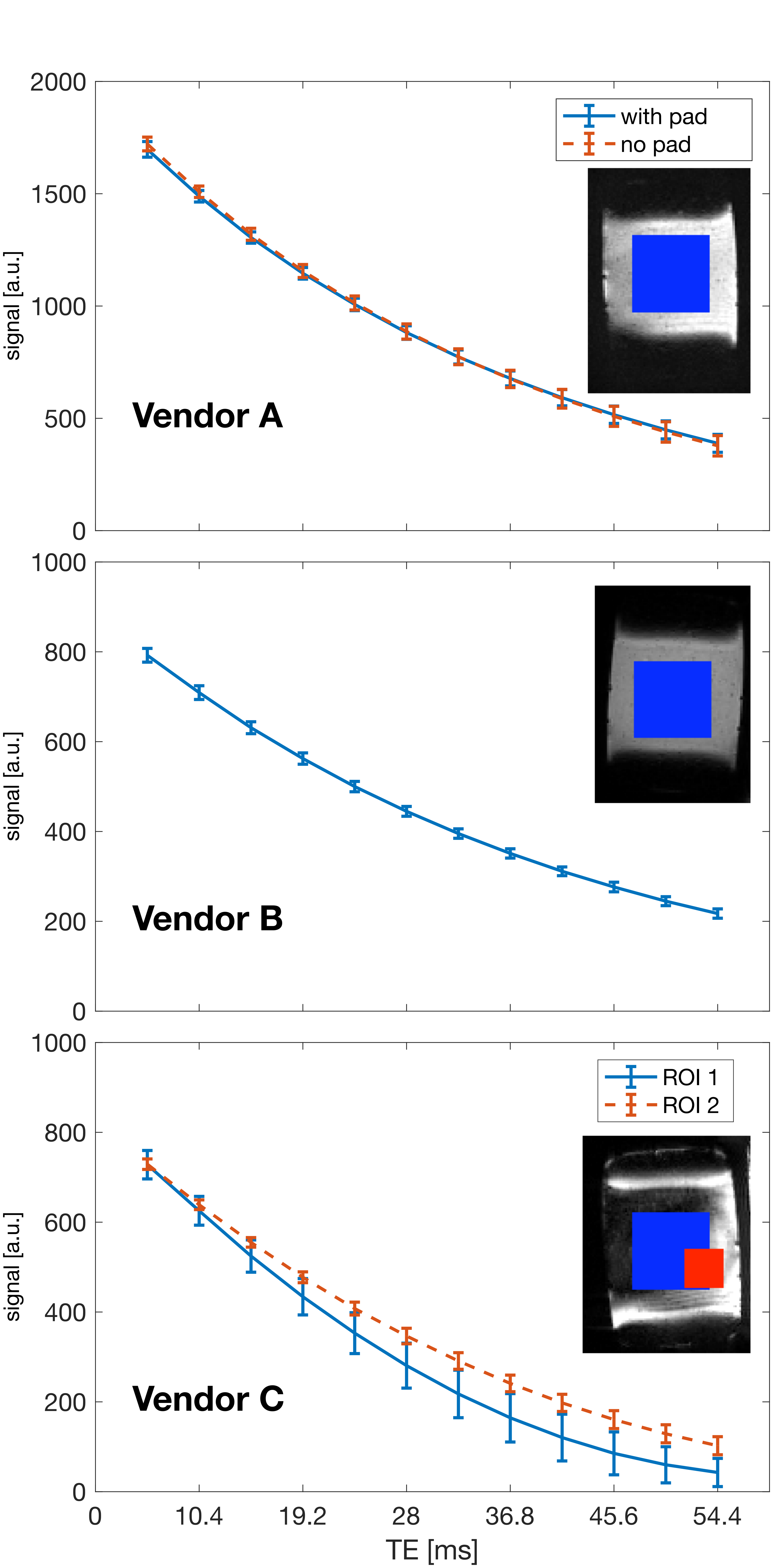
Fig 1 shows the signal decay versus echo time in a square ROI in the phantom. On vendors A and B, the decay is close to exponential, while in vendor C the curves deviate from an exponential curve. On closer inspection, the images from vendor C show large regions of signal loss at higher echo times compared to vendors A and B. A second, smaller, ROI was drawn on the last-echo image in a region containing signal, and is showing signal decay closer to exponential decay.

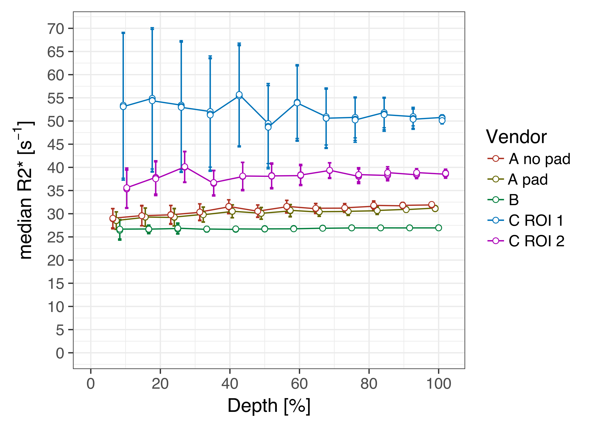
In fig 2, the R2* relaxation rate is shown as function of the depth. Mean R2* [s^-1] over all the layers is 28.5 for vendor A with dielectric pad, 30.8 without using the pad, 26.8 for vendor B, 52.1 for vendor C and 38.2 for vendor C in ROI 2. R2* standard deviations for vendor C are considerably larger than in vendors A and B.

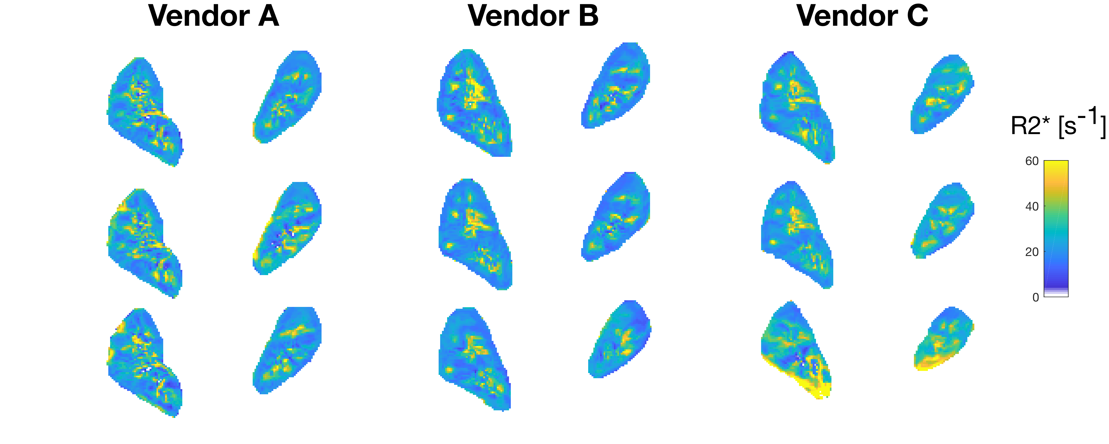
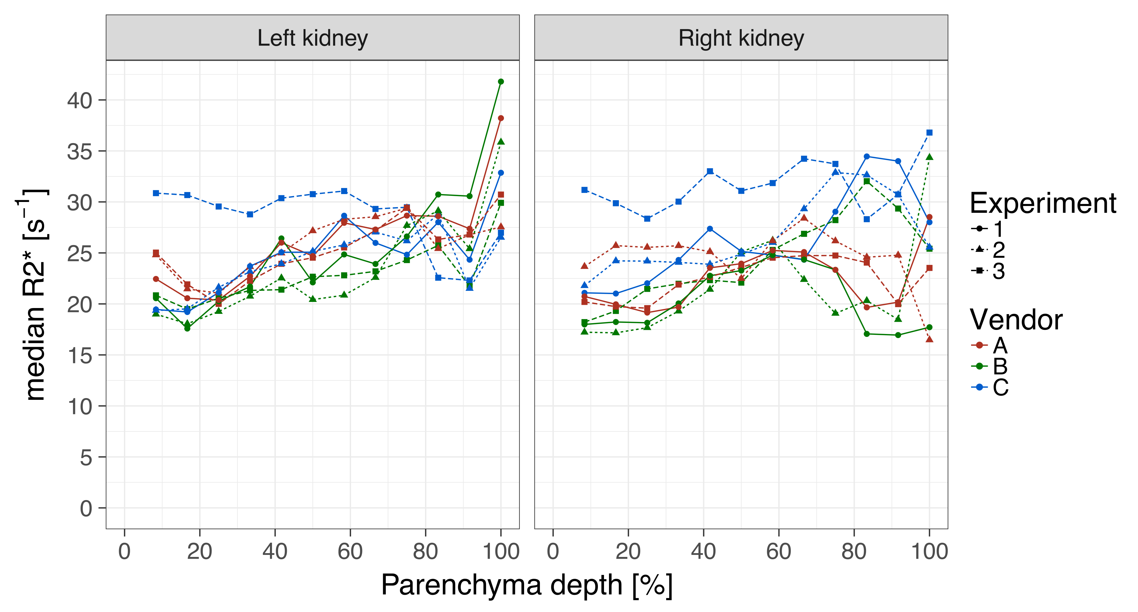
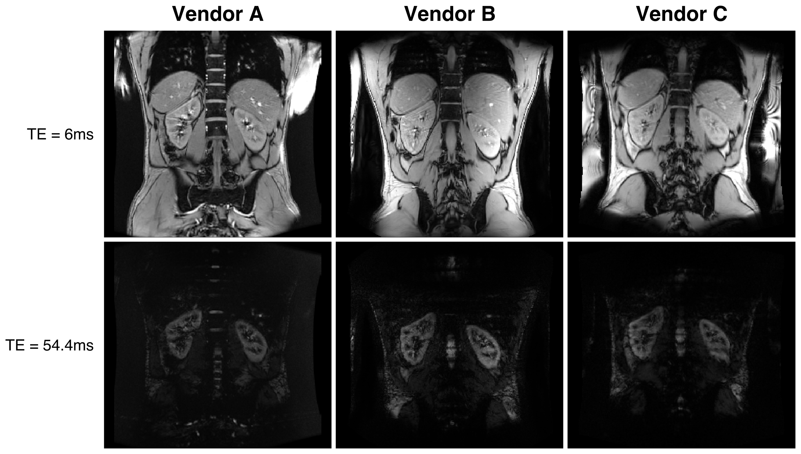
In the volunteer, R2* maps across three vendors are visually similar as shown in fig 3. The concentric layer method shows that R2* values between the three scanners are in the same range (Fig 4), but deeper layers show large variations. R2* values for the left and right kidney are similar for all vendors, while for vendor C the values are higher in one of the experiments. GRE images, Fig 5, at TE=6 and TE=54.4 ms show comparable image quality for vendors A and B, but show artefacts and signal loss in vendor C.

Discussion/Conclusion

Acknowledgements

References