4496
Two compartment fitting for Luminal Water Imaging: multi-echo T2 in Prostate Cancer1Centre for Medical Imaging, University College London, London, United Kingdom, 2Department of Radiology, University College London Hospital NHS Foundation Trust, London, United Kingdom, 3Centre for Medical Image Computing, University College London, London, United Kingdom
Synopsis
This work aims both to show that using a constrained fitting method for Luminal Water Imaging with fewer echoes produces accurate parameter estimates and that this fitting method is feasible for detecting and grading Prostate Cancer. Simulated signals were produced and the mean LWF across multiple iterations was calculated for two models. Then 19 patients were imaged and the images were contoured in both cancerous and benign regions. The simulation showed that the proposed constrained method is accurate and the in-vivo imaging reinforced the idea that multi-echo T2 modelling shows promise in detecting and grading PCa.
Introduction
Similar to methods developed for imaging myelin in the brain1, Luminal Water Imaging (LWI), a fitting technique for multi-echo T2 data recently proposed by Sabouri et al.2, calculates the percentage volume of lumen within a voxel. LWI has been shown to be closely related to the luminal space in prostatic tissue2, with a recent study demonstrating the feasibility of luminal water imaging in the detection and grading of PCa3. However, the current method requires a 64-echo acquisition which is time consuming and may not be available without dedicated scanner research software. This work seeks to show that the combination of an appropriately refined fitting method and fewer acquired echoes provide values of the Luminal Water Fraction (LWF) that are in close agreement with those of the original LWI. Correlations to Gleason score were then performed along with the AUC, sensitivity and specificity of the detection of PCa.Methods
Model The original fitting proposed by Sabouri et al1 used a smoothed non-negative least squares (NNLS) fitting over many variables to produce a distribution $$$p$$$ of T2 values4. The method proposed here constrains this distribution to consist of two Gaussians. This constraint was imposed because the vast majority of voxels in the Sabouri studies2,3 showed two main signal components, which may provide a more robust fitting. The model relating the Signal $$$S$$$ to the distribution $$$p$$$ of T2 values is: $$S = M_0 \int_{0}^{\infty}p(T2)exp(-\frac{TE}{T2})dT2$$ where $$$M_0$$$ is the overall magnitude of the signal and $$$TE$$$ is the echo time. For each voxel six parameters were estimated: overall scaling ($$$M_0$$$), relative fraction between the two compartments (α), mean and standard deviation of the short T2 peak (μ1 and σ1) and mean and standard deviation of the long T2 peak (μ2 and σ2). The LWF was calculated as the area under the long T2 component divided by the area under both components.
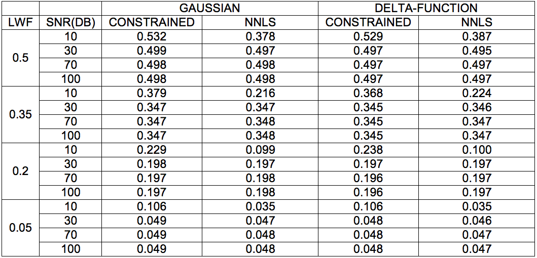
Simulation Simulated signal decays were produced for two separate underlying T2 distributions (two delta functions at T2short and T2long and two Gaussian distributions with means T2short and T2long, fixed at T2short = 75ms and T2long = 600ms) with varying values of LWF, Signal-to-Noise Ratio (SNR) and Number of Echoes (NE). For each combination of parameters 50 iterations of the signal were created. For each iteration the original and new fitting methods were tested using 64-echo and 32-echo simulation signals respectively. The mean LWF across the 50 iterations was then calculated for both models in order to show how the two compare over a range of LWF and SNR values.
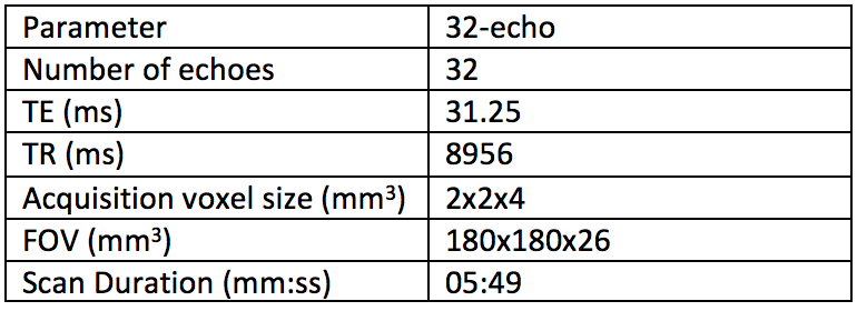
Data In order to investigate the relationship between this new fitting method and Gleason Score, 19 subjects were imaged for this study. The scan parameters are included in Figure 1. A board-certified radiologist contoured 15 lesions in 19 patients, which were confirmed to be cancers following targeted biopsy. Regions of interest (ROIs) were also placed in 16 areas of normal tissue in each of the subjects, all of which were histologically confirmed as benign.
Statistics A Spearman’s rank correlation test was used to find the correlation between Gleason Score and LWF and the Area Under the Curve (AUC), sensitivity and specificity values were calculated using a Receiver Operating Characteristic (ROC) analysis with 5-fold cross validation to reduce problems arising from multiple ROIs coming from the same image.
Results
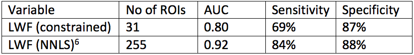
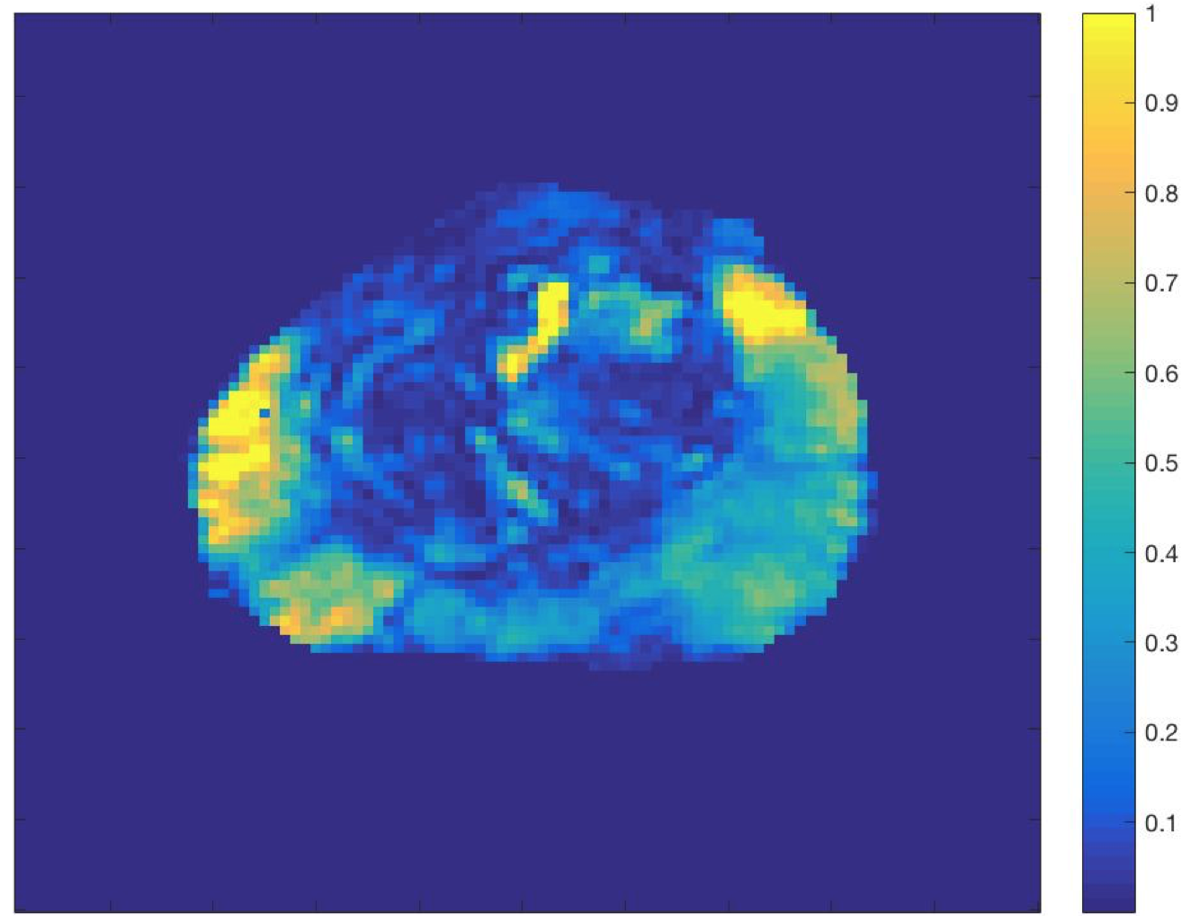
Figure 1 shows the scan parameters of the 32-echo acquisition. Figure 2 shows that for nearly all values of LWF and SNR, using either the delta function or Gaussian assumption, the LWF value produced by the new method is at least as accurate as the original. Using a Spearman’s rank correlation test a correlation of -0.667 was found between Gleason Score and LWF in 31 ROIs. Figure 3 shows the AUC, sensitivity and specificity achieved by the new fitting method in 31 ROIs. Figure 4 is an example LWF map of the prostate. Note the higher LWF in the peripheral zone (PZ), consistent with histological findings of large regular acini and loosely woven stroma in the PZ5.Discussion
The LWF values calculated in simulation using both fitting methods show that the new constrained method is just as accurate as the original. The correlation between Gleason Score and LWF then reinforces the idea that multi-echo T2 modelling shows promise as a method for detecting and grading PCa. The AUC, sensitivity and specificity of the detection of PCa are all lower in this study when compared to previous results6 but this may be down to a much lower number of ROIs.Conclusion
This new method shows promise in being able to significantly reduce the number of measurements needed to carry out LWI, making it a more clinically viable method.Acknowledgements
Cancer Research UK through the Comprehensive Cancer Imaging Centre, Prostate Cancer UK and the NIHR funded biomedical research centre at UCLH.References
- Whittall K., et al. "In vivo measurement of T2 distributions and water contents in normal human brain." Magnetic Resonance in Medicine 37, no. 1 (1997): 34-43.
- Sabouri S., et al. “MR Measurement of Luminal Water in Prostate Gland: Quantitative Correlation Between MRI and Histology.” Journal of Magnetic Resonance Imaging 46, no. 3 (2017): 861-869
- Sabouri S., et al. “Luminal Water Imaging: A New MR Imaging T2 Mapping Technique for Prostate Cancer Diagnosis” Radiology 284, no. 2 (2017): 451-459
- Bjarnason T., et al. “AnalyzeNNLS: Magnetic resonance multiexponential decay image analysis” Journal of Magnetic Resonance 206, (2010): 200–204
- McNeal J. “Normal Histology of the Prostate” The American Journal of Surgical Pathology 12, no. 8 (1988):619-633
- Sabouri S., et al. “Luminal water imaging: a
novel MRI method for prostate cancer diagnosis” Proc. Intl. Soc. Mag. Reson. Med. 24 (2016) 2489
Figures