4482

Linear binning maps for image analysis of pulmonary ventilation with hyperpolarized gas MRI: transferability and clinical applications

Guilhem Jean Collier¹, Laure Acunzo¹, Laurie J Smith^1,2, Paul J Hughes¹, Graham Norquay¹, Ho-Fung Chan¹, Alberto M Biancardi¹, Helen Marshall¹, and Jim M Wild¹

¹Academic Radiology, University of Sheffield, Sheffield, United Kingdom, ²Sheffield Children’s Hospital NHS Foundation Trust, Sheffield, United Kingdom

Synopsis

This work applies a clustering method developed for image analysis of lung ventilation with hyperpolarized ¹²⁹Xe to data acquired in a different centre with ¹²⁹Xe and ³He. Results show that the current method is not readily transferable using published reference values. A different normalization method that increases the reproducibility of ventilation categorization is proposed. After optimization, the technique was applied in groups of patients with chronic obstructive pulmonary disease and cystic fibrosis. Results show significant differences of ventilation distribution indices between patient and healthy control groups.

Introduction

Pulmonary MR imaging with hyperpolarized (HP) ³He and ¹²⁹Xe enables the direct visualization of gas distribution in the lungs and has been used to study the heterogeneity of regional ventilation.^1-3 The ventilation defect percentage (VDP) is the standard outcome metric that describes only the proportion of un-ventilated regions of the lung. In an effort to quantify the ventilation distribution in its entirety, a clustering method producing linear binning maps for ventilation images with HP ¹²⁹Xe has been proposed.^4,5 This work aims to reproduce this method and apply it to HP ³He and ¹²⁹Xe images of healthy controls acquired at a different imaging centre, and to evaluate if results are consistent with published optimum parameters. We also propose an alternative normalization method to rescale the histograms, and study the reproducibility and applicability of both methods in different patient populations.

Methods

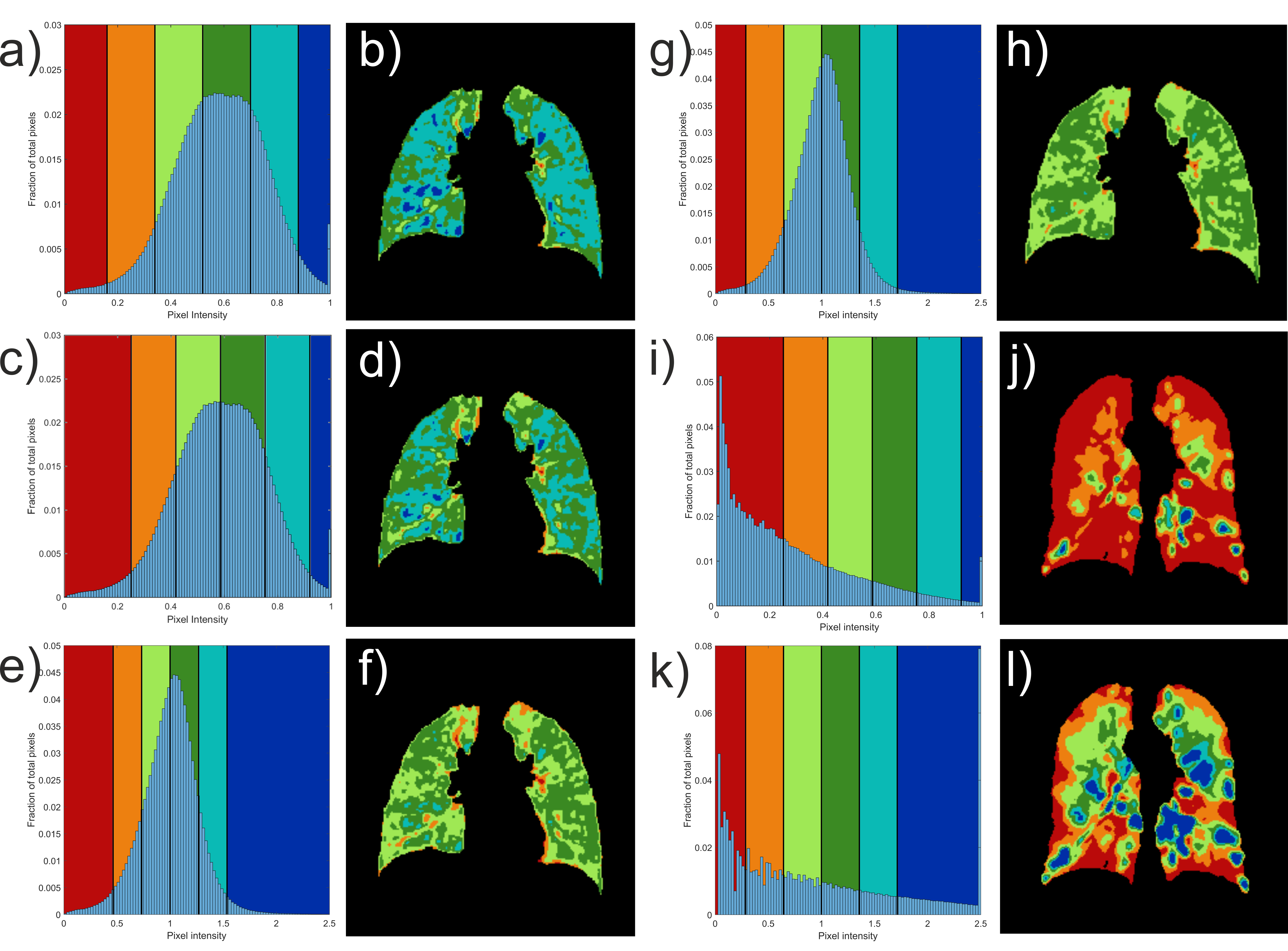
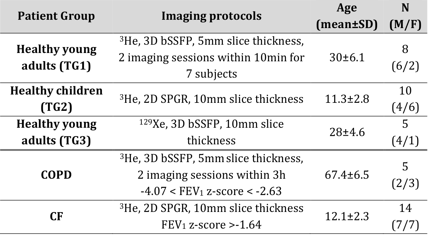
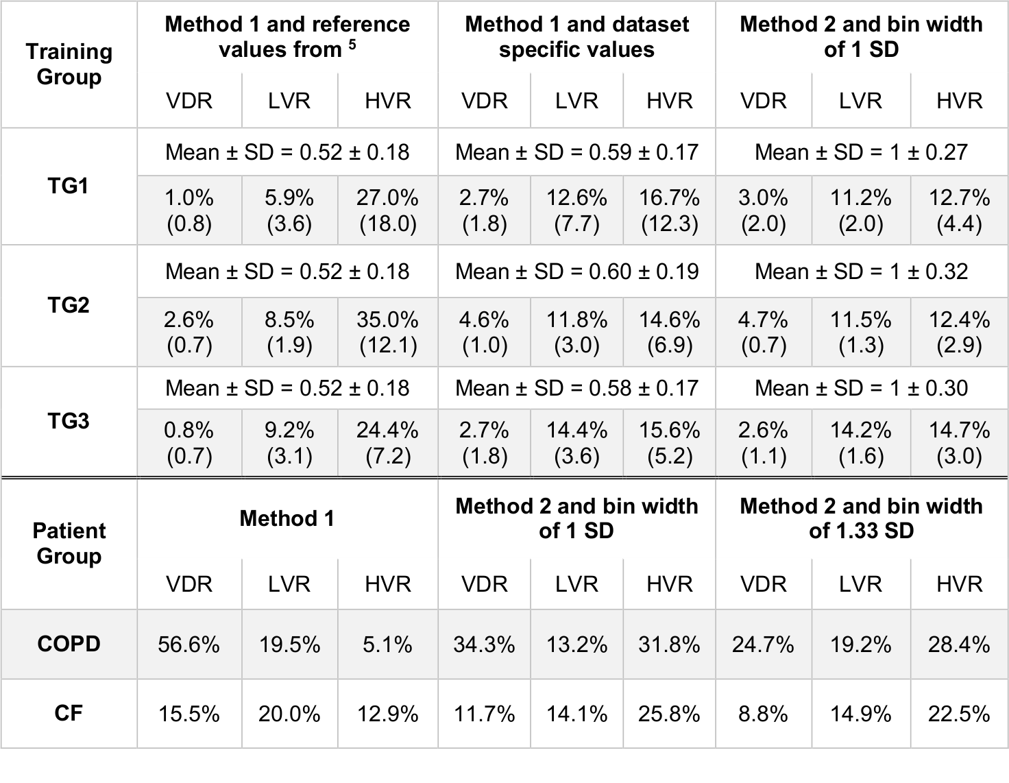
All imaging protocols were performed on a 1.5T GE HDx MR scanner. Three training groups of healthy subjects (TG1-3) and 2 groups of patients with COPD and mild cystic fibrosis (CF) underwent ventilation imaging with HP gas and anatomical ¹H structural imaging (see Table 1). Images were analysed following the methods published previously ⁵ with the difference that the vesselness filter correction was not implemented. After correcting for bias field inhomogeneity and normalizing by the top percentile of the intensity distribution (method 1), histograms were divided into 6 bins and merged into 4 categories: ventilation defect region (VDR, 1^st bin), low ventilation (LVR, 2^nd bin), normal range (NR, 3^rd and 4^th bins) and high ventilation (HVR, 5^th and 6^th bins). An alternative normalization procedure was also evaluated, consisting of scaling the histograms by the mean signal inside the lung cavity mask excluding the airways (method 2). Average histograms for each of the three training groups were generated and the corresponding mean and standard deviation (SD) were calculated. The 6 bins were centred around the mean value and have a common width of 1 SD. Binning maps were produced and VDR was compared to VDP measurement using spatial fuzzy C-means segmentation ⁶ in the COPD patient group. Additionally, the bins width of method 2 was empirically optimized to match VDP ⁶, treated as the gold standard in this study. Reproducibility analysis was performed with Bland Altman on subjects who underwent two MRI sessions (Table 1).

Results

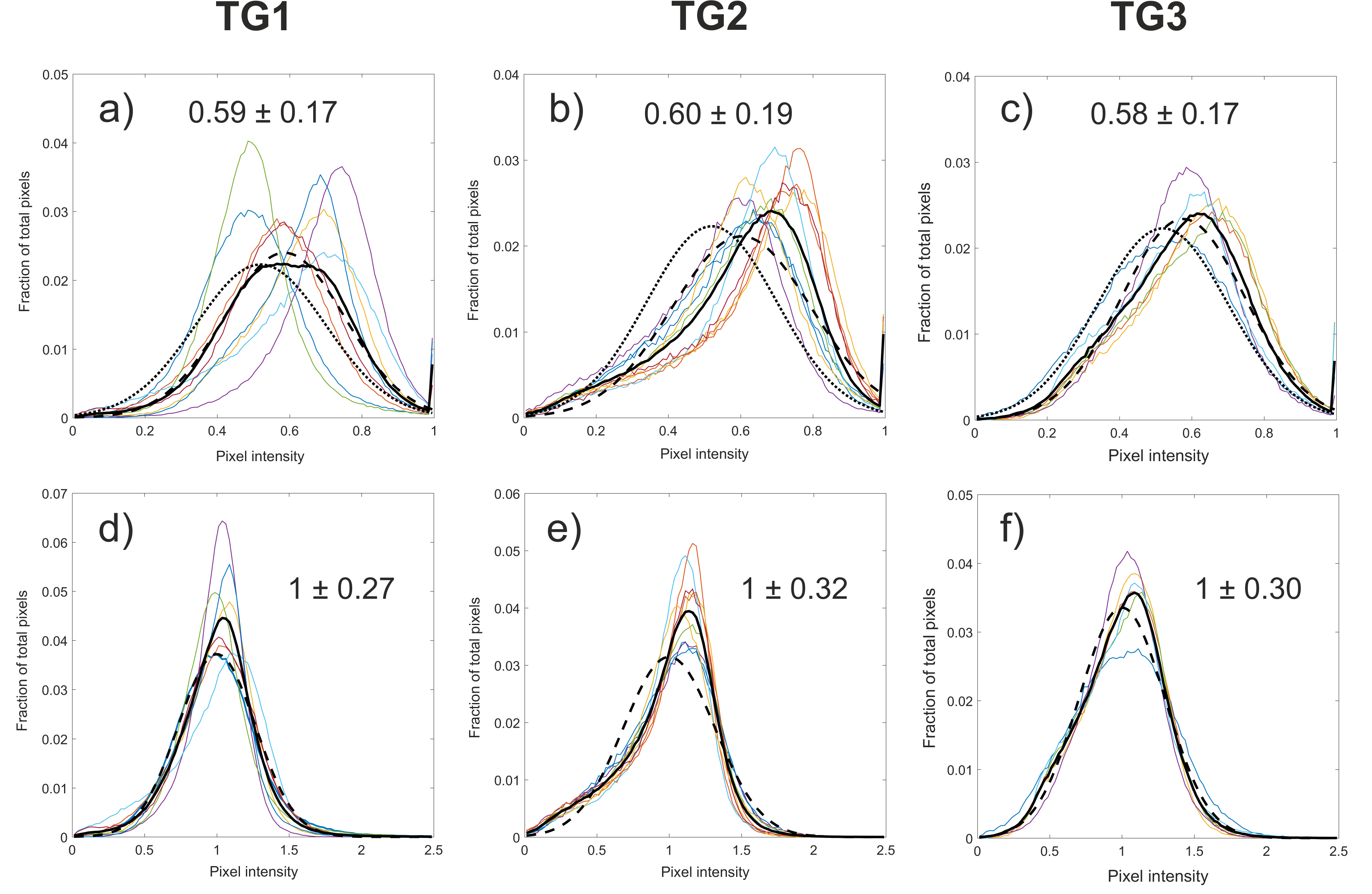
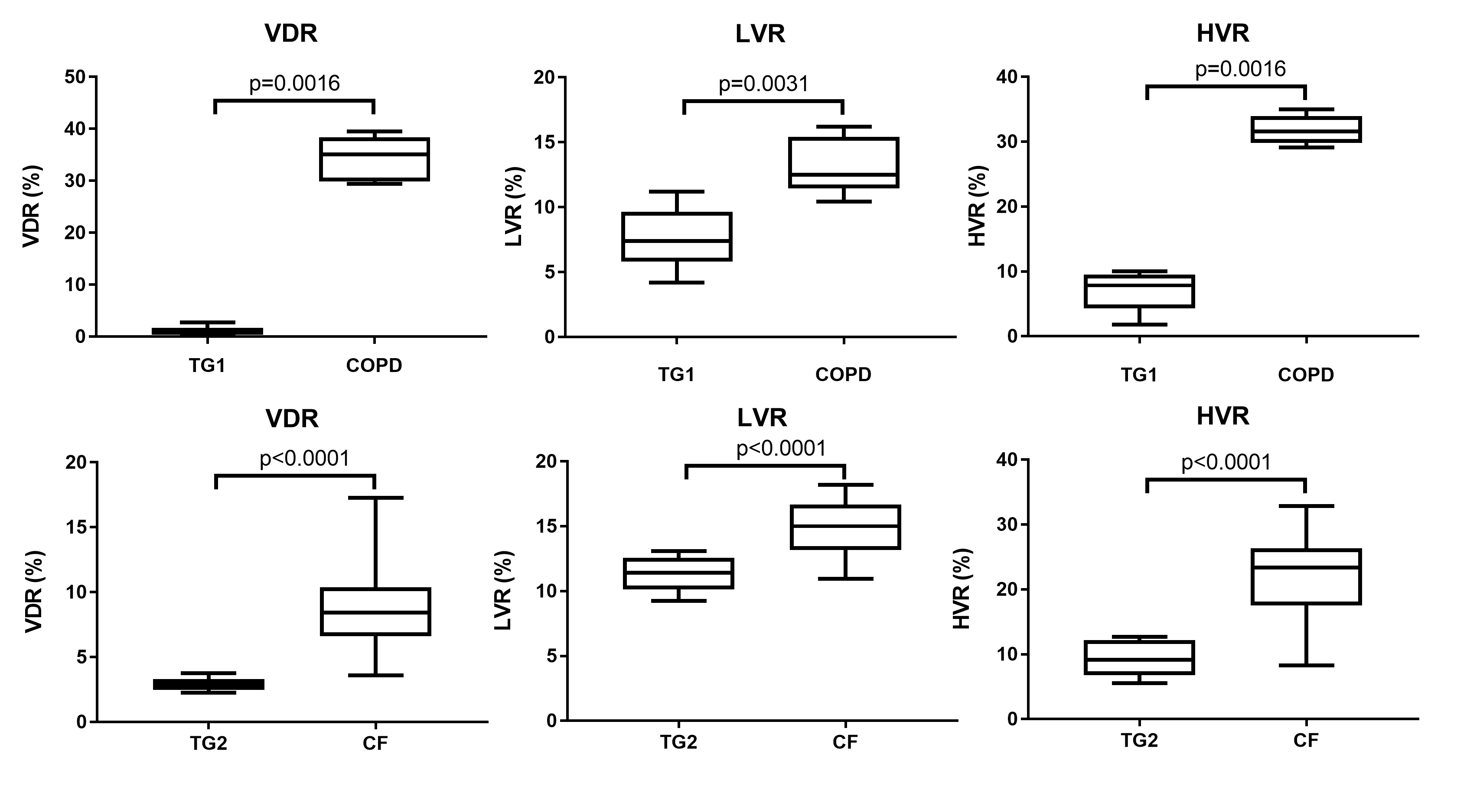
Average rescaled histograms are displayed in Fig.1 for each training group. Histograms using method 1 were consistently shifted toward a higher mean value compared to the published reference data of 0.52±0.18 (mean±SD).⁵ When using these latter values, a higher HVR was consistently obtained compared to the derived training group specific values (Fig. 2 and Table 2). The width of the first bin interval however, was wider when using training group specific values (Fig.2 c) & i)). Method 2 resulted in higher similarity between individual and average histograms for each training group (Fig.1) and it had a lower variability within each reference group (see category SD values in Table 2). It also showed higher reproducibility with lower 95% limits of agreement of (-12.9%, 12.5%), (-1.2%, 2.3%), (-15.8%, 13.4%), (-6.4%, 8.0%) for VDR, LVR, NR and HVR respectively compared to (-27.5%, 30.1%), (-6.5%, 10.2%), (-28.5%, 22.1%), (-12.6%, 12.7%) for method 1. Individual and average distributions were not normal. When applied to the two patient groups, both methods resulted in VDR overestimating VDP (Table 2). The empirically-tuned bin width of 1.33 SD in method 2 matched VDR to VDP ⁶ and the effect is highlighted in Fig.2. VDR, LVR and HVR increased significantly in both patient groups when compared to controls training groups (Fig.3).

Discussion

Compared to other published methods for VDP calculation, the linear binning maps have the advantage of defining areas of low and high ventilation. It is not surprising that reference values for defining these areas might be different between centres using different gases and/or imaging parameters. The proposed normalization by the mean takes the average value (corresponding to a theoretical case of total and ideal gas mixing in the lung) as the reference. This value is independent of lung inflation, breathing manoeuvre, gas quantity and polarization, and so may be more transferable between imaging centres.

Conclusion

We propose an alternative normalization method that gives more reproducible measurement of ventilation categories and higher similarity of distribution within each reference group. After optimizing category intervals using imaging protocol specific reference groups, the method was able to differentiate significant differences between ventilation distribution in healthy and disease groups.

Acknowledgements

This work was supported by NIHR grant NIHR-RP-R3-12-027 and MRC grant MR/M008894/1. The views expressed in this work are those of the author(s) and not necessarily those of the NHS, the National Institute for Health Research or the Department of Health.

References

1. Tzeng YS, Lutchen K, Albert M. The difference in ventilation heterogeneity between asthmatic and healthy subjects quantified using hyperpolarized 3He MRI. J Appl Physiol (1985) 2009;106(3):813-822.

2. Kirby M, Svenningsen S, Owrangi A, Wheatley A, Farag A, Ouriadov A, Santyr GE, Etemad-Rezai R, Coxson HO, McCormack DG, Parraga G. Hyperpolarized 3He and 129Xe MR imaging in healthy volunteers and patients with chronic obstructive pulmonary disease. Radiology 2012;265(2):600-610.

3. Svenningsen S, Kirby M, Starr D, Coxson HO, Paterson NA, McCormack DG, Parraga G. What are ventilation defects in asthma? Thorax 2014;69(1):63-71.

4. He M, Kaushik SS, Robertson SH, Freeman MS, Virgincar RS, McAdams HP, Driehuys B. Extending semiautomatic ventilation defect analysis for hyperpolarized (129)Xe ventilation MRI. Acad Radiol 2014;21(12):1530-1541.

5. He M, Driehuys B, Que LG, Huang Y-CT. Using Hyperpolarized 129Xe MRI to Quantify the Pulmonary Ventilation Distribution. Acad Radiol 2016;23(12):1521-1531.

6. Hughes PJC, Horn FC, Collier GJ, Biancardi A, Marshall H, Wild JM. Spatial fuzzy c-means thresholding for semiautomated calculation of percentage lung ventilated volume from hyperpolarized gas and 1 H MRI. J Magn Reson Imaging 2017.

Figures

Figure 1: Individual (coloured lines) and average (black solid) histogram counts of ventilation intensity within the thoracic cavity mask for the 3 training groups TG1 (a and d), TG2 (b and e) and TG3 (c and f). Comparison between normalization of method 1 (top) and method 2 (bottom). The dashed line represents a normal distribution generated with the mean and standard deviation values (inset within figure) derived from the average histogram and the dotted line represents the reference normal distribution published in ⁵ (mean ± SD = 0.52 ± 0.18).

Figure 2: a-h: average histograms for TG1 and corresponding representative binning maps for one healthy control of TG1 generated using method 1 and intervals value from ⁵ (a, b), method 1 and intervals value using training group specific mean (SD) of 0.59 (0.17) (c, d), method 2 and width of 1 SD (0.27) (e, f), method 2 and width of 1.33 SD (1.33x0.27) (g, h). i-l: average histograms for the 5 patients with COPD and corresponding representative binning maps (from a patient with VDP=20.1%) generated using method 1 (i, j) and method 2 and width of 1.33 SD (k, l).

Figure 3: Top (Bottom): Comparison of ventilation parameters between healthy adult reference databases TG1 (TG2) and the group of patients with COPD (CF) who underwent the same imaging protocol. p values from Mann-Whitney unpaired t-test are reported. There was a signifant difference for each category.

Table 1: Patient demographics and imaging protocols

Table 2: Summary of the intensity distribution per category in the three healthy reference datasets and the two patient groups. Values are given as average (SD) in each group. On average, lower standard deviation values were obtained for method 2. The quoted “Mean ± SD” values represent the mean and standard deviation values calculated for the average histogram of the training group that were used for calculating the bins’ intervals. Reference values from TG1 (TG2) were used for COPD (CF) groups. For comparison, patients with COPD (CF) had a mean VDP ⁶ of 25.9% (10.8%).

Proc. Intl. Soc. Mag. Reson. Med. 26 (2018)

4482