4426
Development of a field camera system for a customized 1.5 T compact MRI system1University of Tsukuba, Tsukuba, Japan
Synopsis
We developed a field camera system for a 1.5T/280mm superconducting magnet system with unshielded gradient coils. K-space trajectories of a two-dimensional spiral scan were monitored using the field camera system and predicted based on a gradient impulse response function (GIRF). Image reconstruction with these trajectories was effective to recover artifact-free images, even in the presence of hardware imperfections. This result showed the validity of the system.
Introduction
Stable and homogeneous magnetic fields and accurate k-space trajectories are essential to high quality MR images. However, in many cases, it is difficult to establish such ideal conditions for MR image acquisition. To overcome these situations, field monitoring devices using many tiny NMR probes (field cameras) were proposed [1,2]. The field camera is especially important for customized MRI systems because it is difficult to optimize the combinations of hardware units such as the magnet, the gradient coils, the RF coils, and the MRI control systems. In this study, we developed a customized field camera for our home-built MRI system using a compact 1.5 T superconducting magnet (280 mm bore) equipped with unshielded gradient coils and evaluated it using spiral trajectories.Materials and Methods
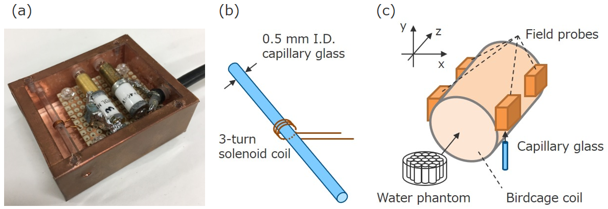
Figure 1(a) shows the 1H-NMR probe developed in this study. The size of the NMR probe was 51 mm (length) × 41 mm (width) × 23 mm (height). The NMR probe consisted of a capillary glass (inner diameter = 0.5 mm) filled with CuSO4-doped water and a 3-turn solenoid coil as shown in Fig.1(b). The probe lifetime was about 30 ms. Figure 1(c) shows our field camera system consisted of an 8-element birdcage coil (diameter = 64 mm, length = 64 mm, shield diameter = 85 mm) and four NMR probes.
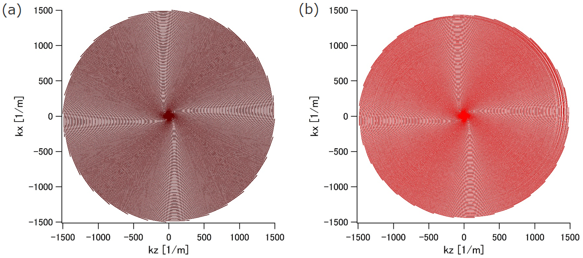
We used a home-built compact MRI system consisting of a 1.5T/280mm horizontal bore superconducting magnet (JMBT-1.5/280/SS, JASTEC, Kobe, Japan), second-order shim coils (diameter = 250 mm), unshielded gradient coils designed with the target field method [3] (diameter = 160 mm, efficiencies: 1.97, 1.92, 2.52 mT/m/A for Gx, Gy, and Gz), the birdcage coil, and a fully-digital MRI console (DTRX6, MRTechnology, Tsukuba, Japan) [4]. A cylindrical water phantom was measured in the z-x plane with a spiral scan sequence (32 interleaves and acquisition time per interleaf = 12 ms) as shown in Fig.2(a).
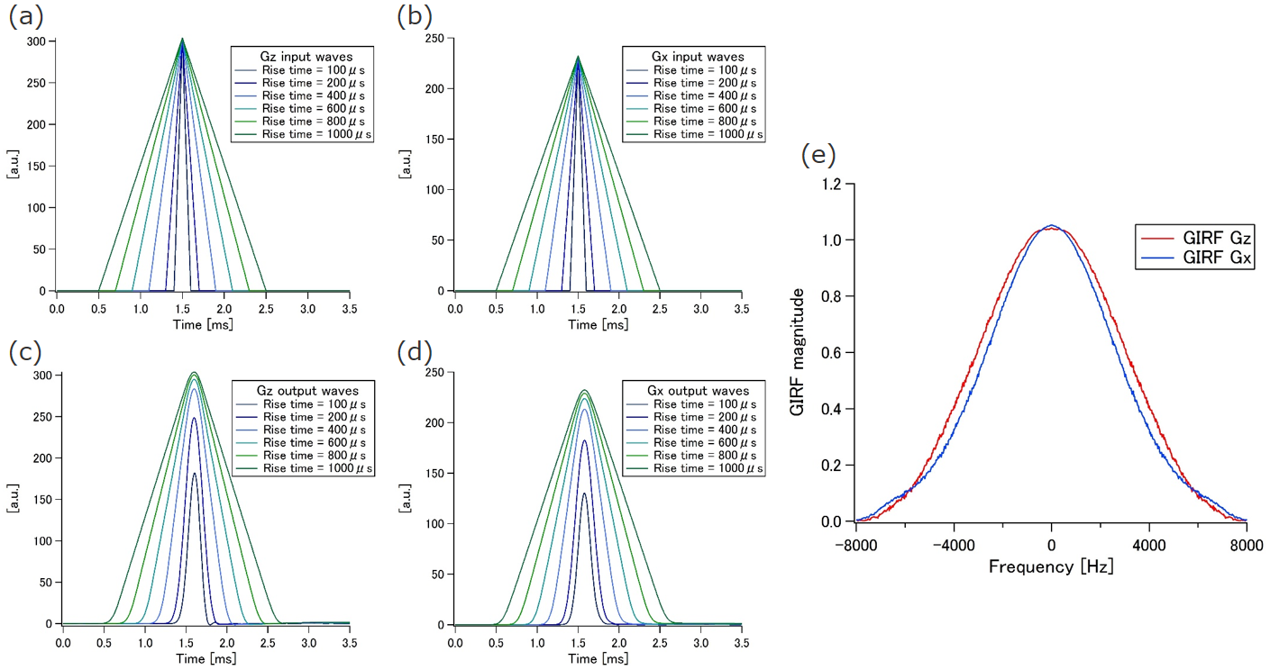
The first correction method was to monitor the k-space trajectory of the spiral scan. The FID signals of the four probes were used to analyze the trajectory and field drift using a first-order spherical-harmonic model with four basis functions [1]. The second correction method was to predict the trajectory considering the hardware imperfections by using the gradient impulse response function (GIRF) [5]. The output o(t) is described by convolution of the input to the system i(t) and the impulse response h(t). This relation can be written as O(ω) = I(ω)H(ω), where O(ω), I(ω), and H(ω) represent the Fourier transforms of i(t), o(t), and h(t), respectively. The system response to any given input can be predicted based on the GIRF H(ω). The field camera system can measure the output of the gradient o(t), which enables to calculate the GIRF. Actually, it is impossible to apply the impulse-type gradient, this measurement was performed by applying the triangle waves (gradient rise time = 100, 200, 400, 600, 800, 1000 µs, and fixed current value = 3 A, Figs. 3(a) and (b)).
Results and Discussion
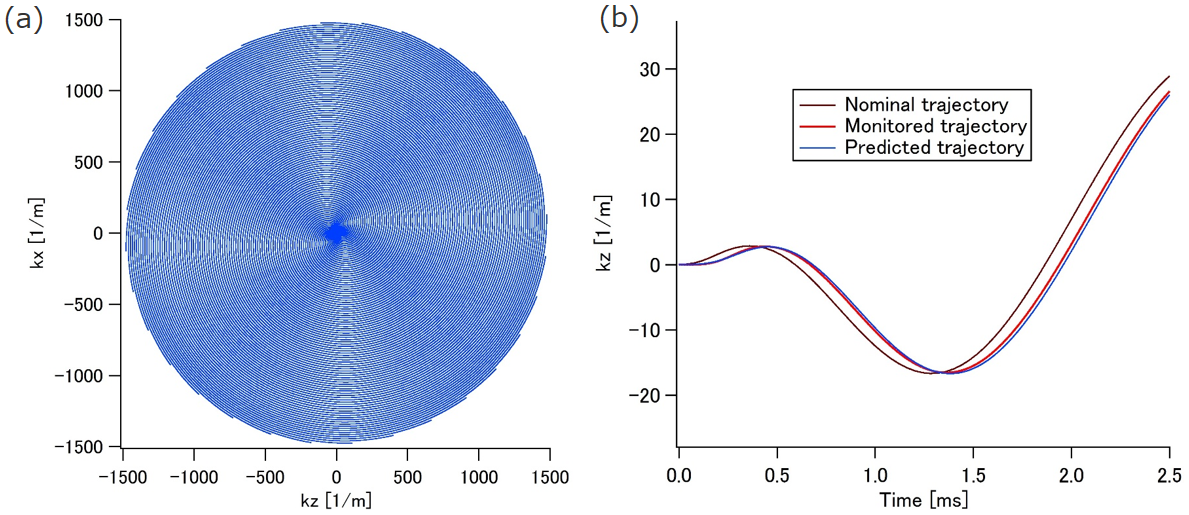
Figures 2(a) and (b) show the nominal and monitored k-space trajectories. Although it appears to have monitored the trajectory properly because these trajectories were much the same, the monitored trajectory was a little smaller than the nominal one, which may be caused by the residual eddy-current fields. Figures 3(c) and (d) show the outputs of triangle waves in z and x directions. The outputs rose later and blunter than the inputs because of the eddy current and the gradient delay. According to the above equation, GIRFs in z and x direction were successfully calculated (Fig. 3(e)). Figure 4(a) shows the predicted trajectory based on the GIRFs. Compared with the nominal trajectory, the monitored and predicted trajectories rose later about 100 µs, which indicated that the gradient delay was reflected correctly. Figures 5(a)-(c) show the phantom images reconstructed with the nominal, monitored, and predicted trajectories, respectively. The artifact was successfully removed in the images reconstructed with the monitored and predicted trajectories. This result showed the validity of the system.Conclusion
In conclusion, our field camera system was successfully installed to our customized 1.5 T compact MRI system and demonstrated its usefulness for image quality improvements.Acknowledgements
No acknowledgement found.References
[1] C. Barmet et al. Spatiotemporal magnetic field monitoring for MR. Magn Reson Med 2008; 60: 187-197. [2] C. Barmet et al. A transmit/receive system for magnetic field monitoring of in vivo MRI. Magn Reson Med 2009; 62: 269-276. [3] Turner R. A target field approach to optimal coil design. J Phys 1986; 19: 147-151. [4] Hashimoto et al. Development of a pulse programmer for magnetic resonance imaging using a personal computer and a high-speed digital input–output board. Rev. Sci. Instrum 83, 053702 (2012). [5] Signe J. Vannesjo et al. Gradient system characterization by impulse response measurements with a dynamic field camera. Magn Reson Med 2013; 69: 583-593.Figures