Purpose

MRI-Linacs provide image-guided, real-time treatment for cancer patients ¹. When a split magnet is used, it is very challenging to generate perfectly linear gradient fields with a split gradient coil system ². Phantom-based image domain correction methods ³ employ a fitting procedure to extract gradient non-linearity (GNL) information, but with a limited number of marker points, the estimation accuracy may be not guaranteed near the imaging boundary area. Electromagnetic (EM) modelling can be used to estimate the gradient field, but the numerically calculated gradient fields do not always match the measured values. In this work, to improve the accuracy of estimating nonlinear gradient fields, a hybrid method that uses a stream function ^4,5 and grid phantom-based measurement ⁶ is developed. The image distortion caused by GNL in MRI-Linac system can then be effectively corrected.

Methods

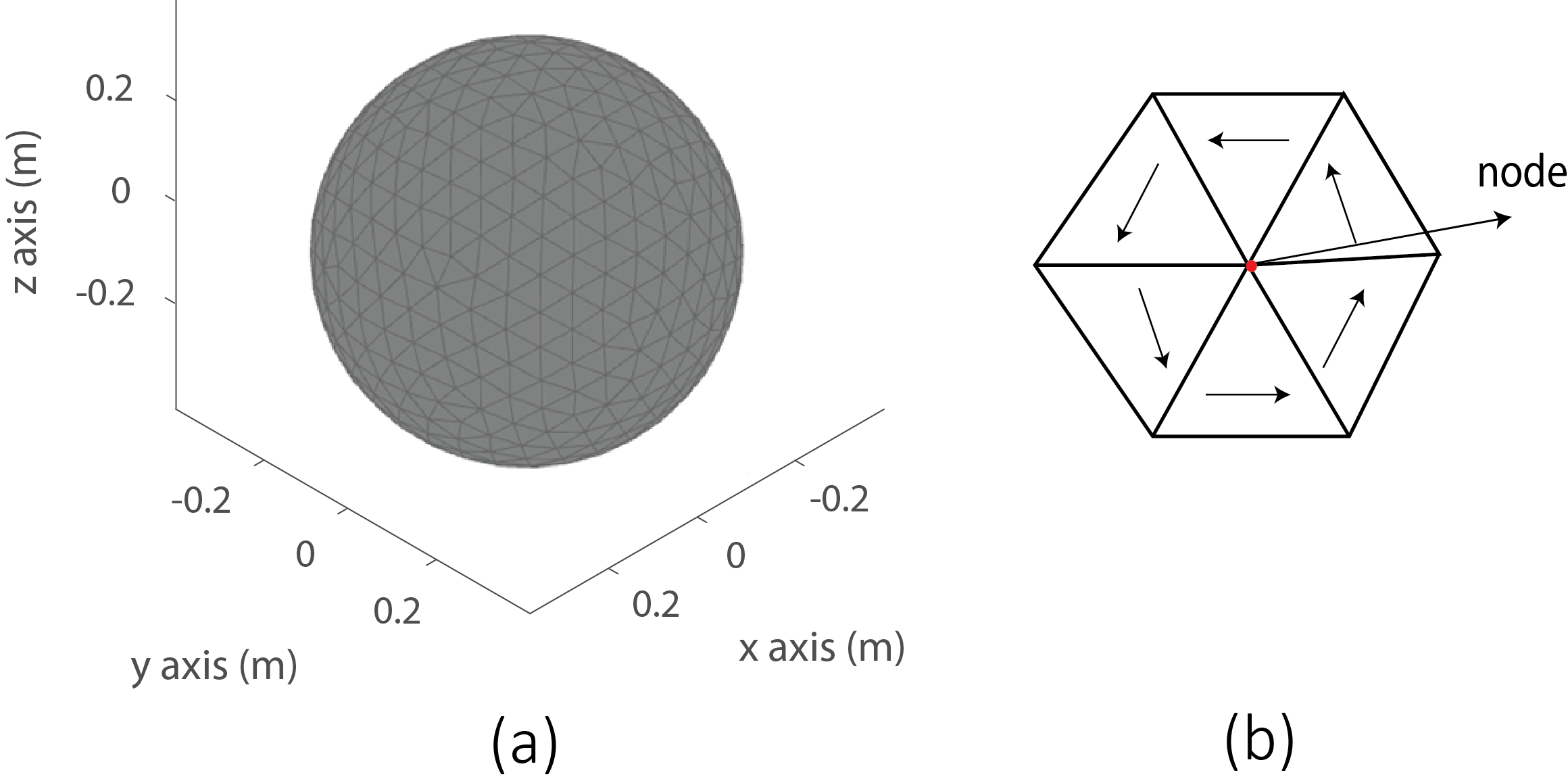
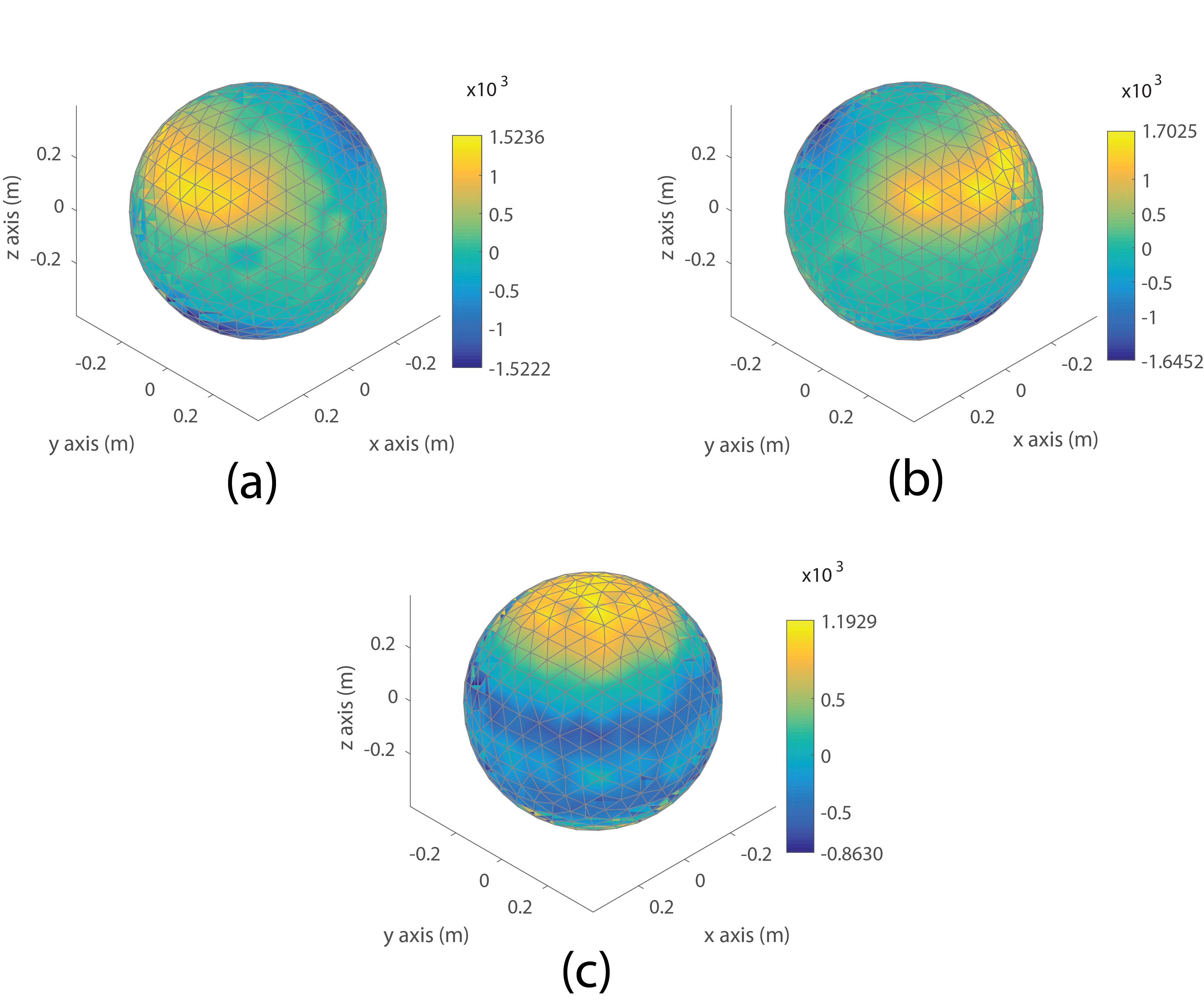
The proposed method corrects GNL in three steps. Step 1: The gradient field profile in the imaging region is acquired via using the grid phantom; Step 2: by means of a stream function method, the current density distribution on a 40 cm diameter sphere is calculated to produce gradient field profile that matches phantom images acquired in step 1. Step 3: with the determined current density distribution, the non-linear gradient fields at any position in the imaging volume can be calculated and used for GNL correction. The kernel of the proposed method is to solve the following optimisation problem:$$ {\mathop{\arg\min}_{\ I_{n\_k}} (\| B(I_{n\_k},r)-B_{k\_nominal}\|_{2}+\alpha W_{magn} \tag{1}}$$where the magnetic field $$${B(I_{n\_k},r)}$$$ at position r was calculated as$$${B(I_{n\_k},r)\approx \frac{\mu_{0}}{4\pi}\sum_{n=1}^N I_{n\_k}\int_{s'} \triangledown \times\frac{f_{n} (r')}{\mid r-r'\mid}ds'}$$$.$$${f_{n} (r')}$$$ denotes the circulating current on the surface of the spherical volume, which is discretised with ‘’elements’’ and N ‘’nodes’’ shown in Figure 1.$$$ I_{n\_k}$$$is the coefficient of the stream function for each node n.$$${\alpha}$$$ is the weight of the magnetic energy, $$${W_{magn}}$$$. According to the phantom mapping from the nominal position$$${r\epsilon C}$$$to the actual position h(r), the magnetic field in measured marker position is calculated as$$${B_{k\_nominal}(r)=G_{k}*h(r)}$$$, where$$$G_{k}$$$ is the k-axis gradient. Once the surface currents on three axes are calculated (shown in Fig. 2) the gradient field at any location inside the 30 cm DSV (Diameter of Spherical Volume) can be calculated for GNL correction (see abstract 5644 of ISMRM 2018 ). Then the undistorted image m can be obtained by solving the following optimization problem:$${\parallel E_{GNL}\cdot Fm-b\parallel_{2} \tag{2}}$$where$$$E_{GNL}$$$ denotes the GNL field encoding, F is the non-distorted Fourier encoding matrix and b is the acquired k-space signal. In this paper, the gradient field and k-space data was simulated according to Liu’s design ². The image size is Nx = Ny = Nz = 256, voxel size is 1mm isotropic.

Results

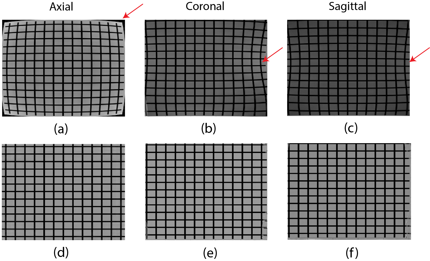
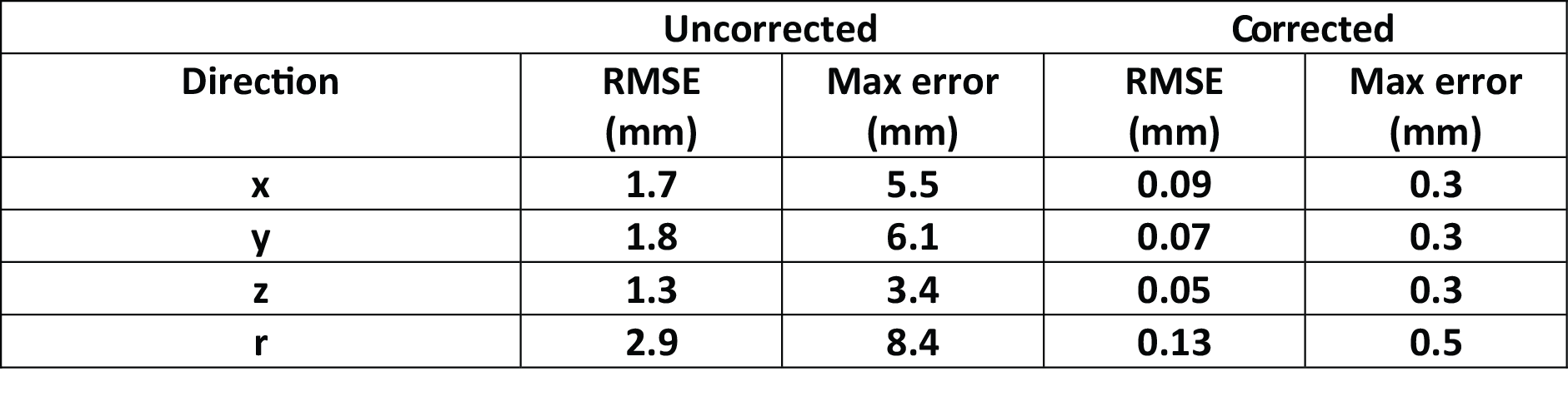
Phantom images before and after GNL correction are shown in Fig. 2 (a-c) and (d-f), respectively. In the top row, geometric distortion is clearly visible before correction, especially at the outer regions denoted with red arrows. However, after applying the proposed method, the geometric distortion caused by GNL is successfully corrected as demonstrated by images (d) to (e) in Figure 2. In Table 1, the root-mean-square-error (RMSE) and the maximum error of the marker coordinates are compared before and after GNL correction. Before correction, the RMSE of marker locations in x, y and z directions was 1.7mm, 1.8mm, and 1.3mm, respectively; with 2.9mm in the positional displacement (r). The RMSE of marker locations in GNL-corrected images decreased significantly to less than 0.15mm. The maximum errors of marker coordinates in x, y and z directions before correction were 5.5mm, 6.1mm, 3.4mm, respectively; with a 8.4mm positional displacement. In comparison, the maximum errors of marker coordinates after GNL correction decreased to 0.5 mm or less, meeting the geometric accuracy requirement of radiotherapy ⁷.

Discussion

Here, the gradient fields and related phantom images were numerically calculated according to our previously designed split gradient coils for MRI-Linac system. The actual gradient fields may have minor deviations from the simulation results. In addition, the gradient field profiles obtained from numerical modelling are usually smoother than those taken from measurement, thus a filtering effect is realized during the implementation of the proposed hybrid method. The practicality of the proposed method will be further validated with experimental data.

Conclusion

In this proof-of-concept work, a hybrid method combining both phantom-based mapping and stream function was proposed for gradient field estimation and GNL-correction in MRI-Linac system. The preliminary simulation results demonstrated that the proposed method can correct GNL-induced image distortions efficiently. In the future, we will verify the proposed method by experiment.

Acknowledgements

No acknowledgement found.