4386
Estimation of prostate cancer distribution on pathology slides via image analysis of IHC-stained slides.1Center for Magnetic Resonance Research, University of Minnesota, Minneapolis, MN, United States, 2Department of Pathology, University of Washington, Seattle, WA, United States, 3Department of Biostatistics, School of Public Health, University of Minnesota, Minneapolis, MN, United States
Synopsis
For the development of CAD systems of prostate cancer, manual annotation of cancer by experienced pathologists is the gold standard for establishing the ground truth. However, the process is tedious and has finite precision. Here, we describe a framework that uses quantitative analysis of IHC-stained slides to derive parameters, which in turn are used by a trained predictive model to estimate the spatial distribution of malignant epithelium. Thresholding of the results provides a reasonable map of cancer that is comparable to manual annotation.
Introduction
There has been significant interest in the development of computational models for detection of prostate cancer (PCa) using multiparametric MRI (mpMRI).1-3 The performance of such models is highly-dependent on the quantity and quality of the modeling data. The gold standard for deriving the ground truth involves the detailed, manual annotation of ex vivo prostate specimens by trained pathologists, followed by co-registration to the imaging data. However, manual annotation of PCa is not only time-consuming, but also prone to error due to finite precision of annotation tools.
A number of recent studies have demonstrated that IHC staining with a triple antibody cocktail (AMACR + HMWCK + p63) can help selectively identify cancerous epithelium. Increased epithelial expression of AMACR is an established marker for PCa,4-5 while the absence of HMWCK and p63, proteins that are selectively expressed by basal cells, is similarly indicative of PCa.6-7 Here, we describe a framework for estimating the spatial distribution of PCa within a slide via semi-automated analysis of triple-stained slides.
Methods
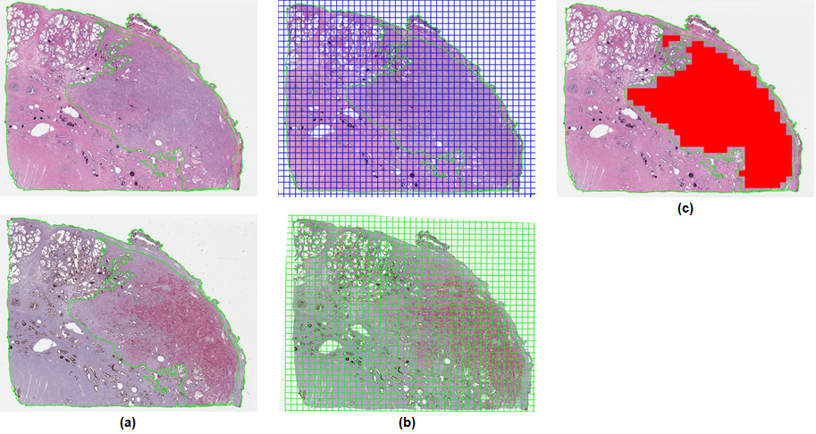
Ten PCa-containing blocks were randomly identified, and adjacent sections were stained for H&E and the triple antibody cocktail, then digitized. PCa was annotated on H&E slides by trained pathologists. SigMap software9 was used to align the adjacent sections, copy the annotated cancer to the IHC slide, and overlay a grid of 0.5 x 0.5 mm analysis squares on both. Analysis squares were labeled cancer if they had ≥75% overlap with the cancer annotation (Fig. 1).
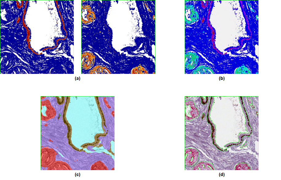
Each analysis square on the IHC slide was analyzed with three algorithms (Image Analysis Toolbox, Aperio). The Color Deconvolution Algorithm (Fig. 2a) separates an image into different color channels (corresponding to different staining components), then quantifies the surface area and optical density (OD) of each stain. The algorithm was configured to quantify both the area and OD of brown staining (HMWCK basal cell marker) and red staining (AMACR marker for cancer epithelium), resulting in 4 outputs of interest. The Coexpression Algorithm (Fig. 2b) was used to calculate the fractional percentages of brown and red staining components in each analysis square (2 outputs of interest). The Genie Classifier Algorithm (Fig. 2c) is a histology pattern recognition algorithm that was trained to predict the percentage of cancer epithelium (among other features) in each analysis square.
40 analysis squares were randomly selected from each triple-stained slide (400 in total) and were manually “hyper-annotated” by pathologists in much greater detail than usual (Fig. 2d). In particular, the percentage of cancer epithelium in each analysis square was determined from the hyper-annotations and taken to be the ground truth.
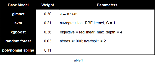
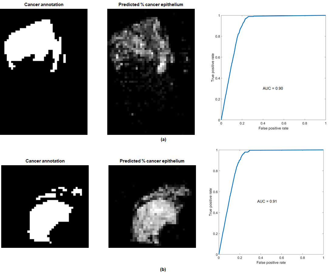
An ensemble regression model was then trained on the 400 hyper-annotated analysis squares to predict the percentage of cancer epithelium in each analysis square, using the 7 outputs of interest from the Aperio analysis algorithms as predictors. Training was performed using the SuperLearner package in R with 5 different base regression models (Table 1). The trained model was applied to all the analysis squares of each triple-stained slide, which produced a map of the predicted distribution of cancer epithelium within a slide. Since thresholding would produce a binary map of cancer, the model was also evaluated using ROC curve analysis via comparison to the (initial) cancer annotation.
Results
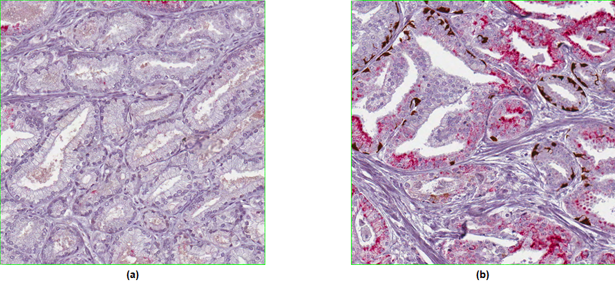
A summary of the trained ensemble regression model is shown in Table 1. The cross-validated R2 value of 0.84 with median absolute error of 2.1 suggests the model produced a good and robust fit. Closer examination of the regression outliers revealed that 2-3% of the hyper-annotated analysis squares had one of two problems with the staining, either cancer epithelium not staining red with racemase as it should (Fig. 3a), or prostatic intraepithelial neoplasia (PIN – a separate entity from PCa) erroneously staining with racemase (Fig. 3b).
Figure 4 shows the results of applying the trained model to an entire slide for two cases. ROC curves obtained via different thresholds for the predicted % of cancer epithelium vs. the annotated cancer are shown as well.
Discussion
The performance of the regression model and the results shown in Figure 4 indicate that the framework for quantitative analysis of triple-stained slides has the potential to supplement or possibly to replace manual annotation of prostate cancer. Inconsistencies in stain uptake as demonstrated in Figure 3 will need to be addressed.Acknowledgements
This work was supported in part by the National Institutes of Health (R01-CA1155268, P41-EB015894, T32-GM008244), Department of Defense (W81XWH-15-1-0477), and the Minnesota Research Evaluation and Commercialization Hub (MN-REACH).References
1. Metzger GJ, Kalavagunta C, Spilseth B, Bolan PJ, Li X, Hutter D, Nam JW, Johnson AD, Henriksen JC, Moench L, Konety B, Warlick CA, Schmechel SC, Koopmeiners JS. Detection of Prostate Cancer: Quantitative Multiparametric MR Imaging Models Developed Using Registered Correlative Histopathology. Radiology. 2016;279(3):805-16.
2. Litjens G, Debats O, Barentsz J, Karssemeijer N, Huisman H. Computer-aided detection of prostate cancer in MRI. IEEE Trans Med Imaging. 2014;33(5):1083-92.
3. Lemaître G, Martí R, Freixenet J, Vilanova JC, Walker PM, Meriaudeau F. Computer-Aided Detection and diagnosis for prostate cancer based on mono and multi-parametric MRI: a review. Comput Biol Med. 2015 May;60:8-31.
4. Rubin MA, Zhou M, Dhanasekaran SM, Varambally S, Barrette TR, Sanda MG, Pienta KJ, Ghosh D, Chinnaiyan AM. alpha-Methylacyl coenzyme A racemase as a tissue biomarker for prostate cancer. Jama. 2002;287(13):1662-70. Epub 2002/04/03. PubMed PMID: 11926890.
5. Luo J, Zha S, Gage WR, Dunn TA, Hicks JL, Bennett CJ, Ewing CM, Platz EA, Ferdinandusse S, Wanders RJ, Trent JM, Isaacs WB, De Marzo AM. Alpha-methylacyl-CoA racemase: a new molecular marker for prostate cancer. Cancer research. 2002;62(8):2220-6. Epub 2002/04/17. PubMed PMID: 11956072.
6. Signoretti S, Waltregny D, Dilks J, Isaac B, Lin D, Garraway L, Yang A, Montironi R, McKeon F, Loda M. p63 is a prostate basal cell marker and is required for prostate development. The American journal of pathology. 2000;157(6):1769-75. Epub 2000/12/07. doi: 10.1016/s0002-9440(10)64814-6. PubMed PMID: 11106548; PMCID: PMC1885786.
7. Wojno KJ, Epstein JI. The utility of basal cell-specific anti-cytokeratin antibody (34 beta E12) in the diagnosis of prostate cancer. A review of 228 cases. The American journal of surgical pathology. 1995;19(3):251-60. Epub 1995/03/01. PubMed PMID: 7532918.
8. Metzger GJ, Dankbar SC, Henriksen J, Rizzardi AE, Rosener NK, Schmechel SC. Development of multigene expression signature maps at the protein level from digitized immunohistochemistry slides. PLoS One. 2012;7(3):e33520
Figures