Synopsis

Active B₀ shimming involves setting currents through a set of shim coils to minimize spatial heterogeneity of B₀ over a prescribed region. This is often phrased as a least-squares problem, based on an acquired field map. Noise in the field map "propagates" and appears as spatially dependent noise in the shimmed field. We show that the shim coils can be characterized by a noise propagation matrix, which is an intrinsic property of the coils and plays an analogous role to the g-factor in sensitivity encoding. This provides a useful metric for investigating the effect of noise in active shimming.

Introduction

Imperfect shimming of the main (B₀) field [1] results from one of two sources of error: shim coils may not offer enough degrees of freedom to capture the spatial variability in B₀(r); and, even if the shims do model B₀ correctly, noise in the field mapping manifests itself as errors in the estimated currents and, hence, in the shimmed field. Herein we address the second source of errors: we present a model for noise propagation in a least-squares shimming solution and investigate its potential for providing a novel metric for assessing its effect on shimming and shim coil design.

Theory

Given j=1,...,N shim coils, each shim coil is characterized by a field per unit current, $$$B_j^{(u)}(\mathbf{r})$$$. Least squares shimming consists of initially "mapping the shim coils" by measuring a matrix C using a homogeneous phantom such that $$$C_{m,n}=B_j^{(u)}\left(\mathbf{r}_n\right)$$$ at M points: $$$\mathbf{r}_1, \mathbf{r}_2, ..., \mathbf{r}_M$$$. Then, once a subject is inside the scanner, a field map $$$\mathbf{b}_k = B_0(\mathbf{r}_k$$$ is acquired. Finally, one solves for N currents, $$$\mathbf{I}=\left( I_1, ..., I_N \right)$$$, which minimize the field variation within the region of interest: $$$||C\mathbf{I} - \mathbf{b}||$$$.The well known least squares solution is $$$\hat{\mathbf{I}} = (C^TV_b^{-1}C)^{-1}C^TV_b^{-1}\mathbf{b}$$$, where $$$V_b$$$ is the spatial covariance matrix of the subject's field map b. The covariance matrix of the resulting difference field $$$\mathbf{d} = \mathbf{b}-C\hat{\mathbf{I}}$$$ is then $$$V_{d}=V_{C\hat{\mathbf{I}}} = CV_IC^T$$$. It is known that, for the general case, $$$V_I=(C^TV_b^{-1}C)^{-1}$$$, and thus: $$$V_d= C(C^T V_b^{-1} C)^{-1} C^T$$$. If we can assume to a first approximation noise is spatially homogeneous within the subject's field map, then $$$V_b=\sigma_b^2 E$$$ and E is the unity matrix; hence:

$$V_d=\frac{\sigma_b^2}{M} D $$

where $$$D\equiv M C (C^T C)^{-1}C^T$$$, M is the number of spatial points and $$$\sigma_b^2$$$ is the spatial variance of the field map (in Hz). The standard deviation in the shimmed region is then:

$$sd(\mathbf{r}_n) = \frac{\sigma_b}{\sqrt{M}} \sqrt{D_{n,n}}$$

The normally distributed error is proportional to the error in the input field maps, $$$\frac{1}{\sqrt{M}}$$$, and the square root of the diagonal of the matrix D. Note that the factor M was actually inserted into our definition of the matrix D to make its value independent of M. This matrix, which we will term the noise propagation matrix, serves an analogous purpose to the "g-factor" encountered in SENSE parallel imaging [2], and is an intrinsic property of the shim coil array.

Methods

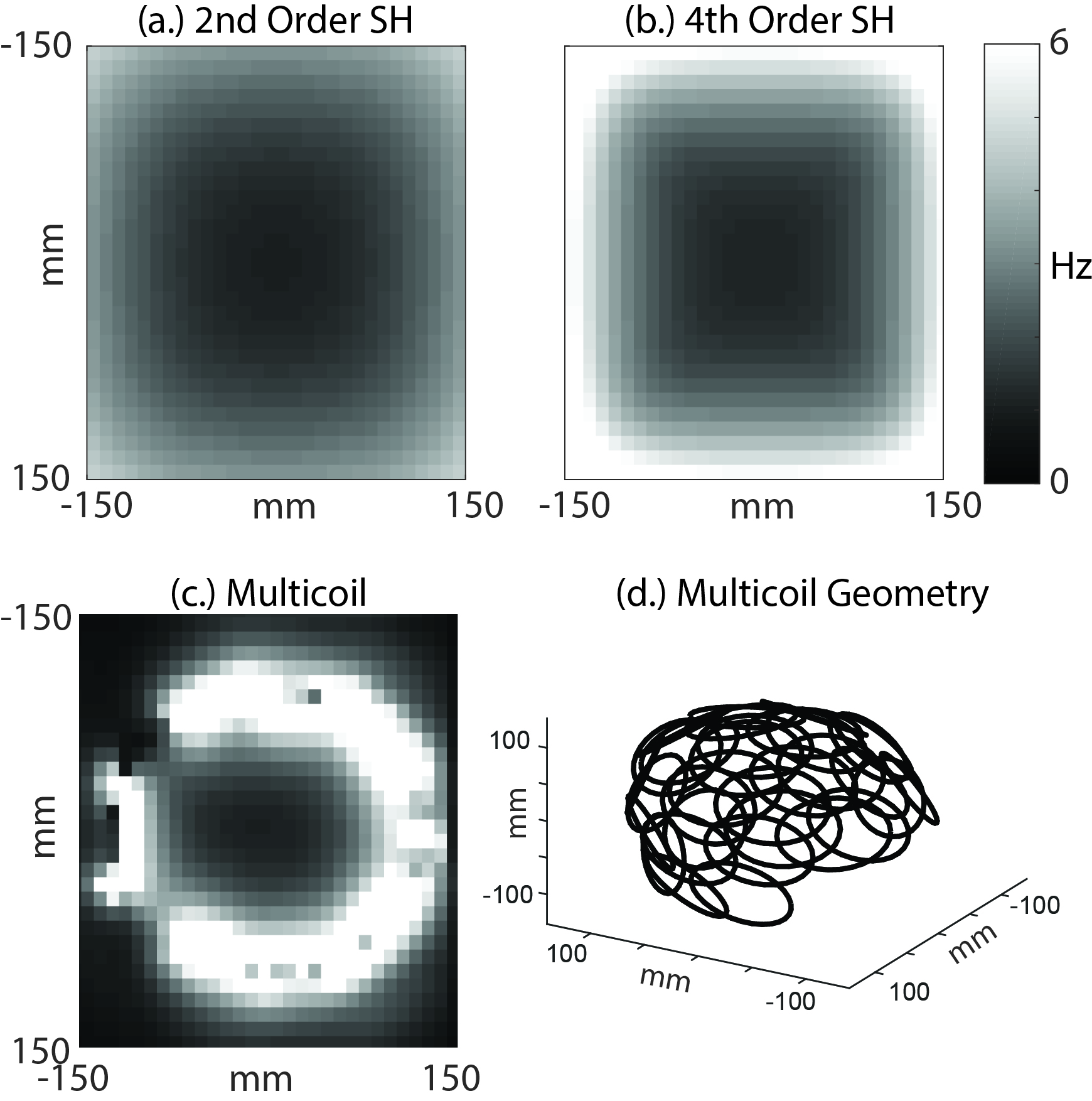
Numerical Simulations: The noise propagation matrix, D, was computed for perfect 2nd order and 4th order spherical harmonic shims, as well for a multicoil shim array as described in [3].

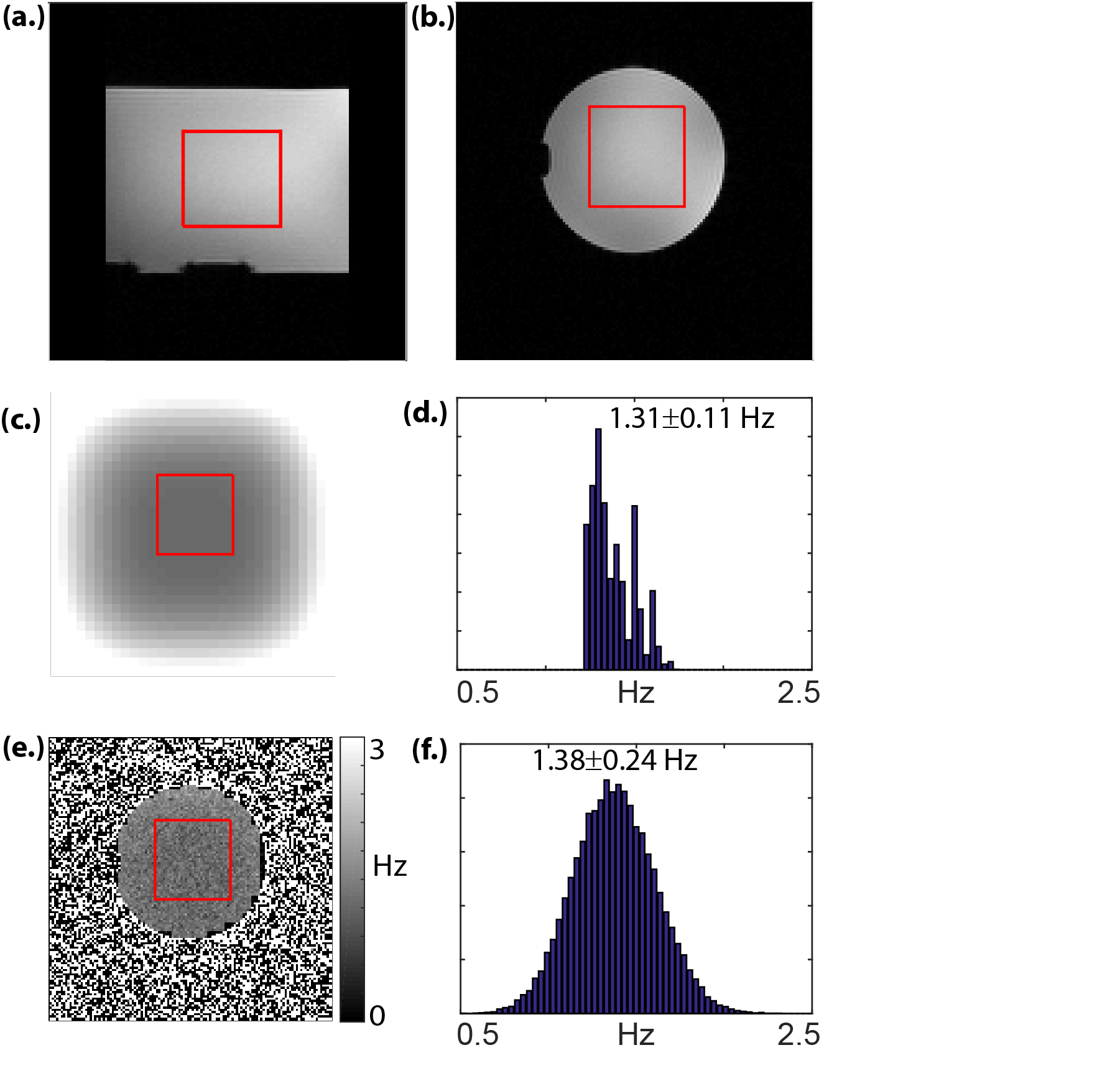
Phantom Experiments: To validate our theoretical prediction for the shimming error, phantom scans were executed on a 3T Tim Trio MRI scanner (Siemens, Erlangen). Double gradient echo field mapping was carried out in an 8-cm radius cylindrical water phantom (TR/TE₁/TE₂=800/4.92/7.32 ms; in-plane FOV 220×220 mm², 128×128 matrix, 70 slices, 2 mm slice thickness, TA=1:42 min, BW per pixel = 1500 Hz). Following field mapping, our in-house shimming least squares algorithm was employed using previously-mapped 1st and 2nd order shim coils. Following shimming, a second field map was acquired for comparison. This procedure was repeated N_rep=12 times, yielding a pre-shimming, post-shimming field and magnitude maps, which were used to estimate the spatial variance in the field maps $$$V_b$$$, and the theoretical prediction for $$$V_d$$$ (after drift correction). The square root of its diagonal was then compared (at each spatial point) to the actual standard deviation in the post-shimming maps, to see how well they agree.

Results

Fig. 1 shows the numerically computed standard deviation in the field post-shimming in a 2D plane through the z=0 coordinate, per unit standard deviation (Hz) and per square root of the number of points in the subject's field map. Both increasing the number of coils and their spatial variability increases the expected deviation, making multicoil arrays, e.g., sensitive near the cortex.

Fig. 2 shows the theoretically predicted (2c) and experimentally computed (2e) spatial standard deviation following shimming, as well as histogram of values from a shimmed VOI (2d, 2f). The means within the shimmed region agree to within 5%. The small discrepancy is attributed to the small number of field maps used to calculate the s.d. (N_rep=12) as well as errors in estimating $$$V_b$$$.

Conclusions

The shim coil noise propagation matrix is an intrinsic property of a shim coil configuration. It can be used to assess a given shim coil configuration. It could also be used to optimize field mapping parameters and examine which spatial regions are more susceptible to the effect of noise in the shimming process.

Acknowledgements

References

[1] Stockmann JP, Wald LL, Neuroimage 2017 (doi:10.1016/j.neuroimage.2017.06.013)

[2] Pruessman KP et al, Magn Reson Med 42:952-962 (1999)

[3] Keil B et al, Magn Reson Med 70:248-258 (2013)