4269
Accelerated Magnetic Resonance Fingerprinting Using Convolutional Neural Network1Center for Biomedical Imaging Research, Department of Biomedical Engineering, Tsinghua University, Beijing, China, 2Department of Diagnostic Radiology, The University of Hong Kong, Pokfulam, Hong Kong
Synopsis
The purpose of this work is to accelerate the acquisition of Magnetic Resonance Fingerprinting (MRF) using Convolutional Neural Network (CNN). Compared with traditional MRF reconstruction using 1000 time points, our CNN model shows better reconstruction fidelity in T2 and similar reconstruction fidelity in T1 using 300 time points. Our study suggests that CNN-based method may be an effective tool in the acceleration of MRF reconstruction.
Introduction
The conventional dictionary matching (DM) in Magnetic Resonance Fingerprinting (MRF)1 was challenged by long computation time, considerable demand for storage and huge round-off errors due to discrete entries of the dictionary. In this study, we demonstrate that Convolutional Neural Network (CNN)2 can be used to significantly reduce the acquisition time of MRF compared to conventional DM without sacrificing the accuracy.Methods
IR-bSSFP was used to acquire MRF signal evolution data with the TR and FA train as shown in Fig. 1. Phase of the excitation pulse alternated by 180° between two consecutive acquisitions. A variable density spiral trajectory was taken for sampling after each excitation pulse. The dictionary was generated using Bloch equation simulations: T1 ranged from 200 to 5000 ms (in an increment of 50 ms), T2 ranged from 1 to 2000 ms (in an increment of 20 ms), and B0 field inhomogeneity ranged from -40 to 40 Hz (in an increment of 1 Hz).
The architecture of CNN model in this study is shown in Fig. 2. The loss function of CNN is defined as $$$\frac{1}{N}\sum\parallel y-\widehat{y}\parallel_{2}+\omega\parallel W\parallel_{2}$$$, where y denotes the true parameters, $$$\widehat{y}$$$ denotes the predicted parameters, ω denotes the regularization parameter, W denotes the weights of CNN, and $$$\parallel\cdot\parallel_{2}$$$ denotes the L2 norm. The first term of the loss function is to enforce fidelity of reconstruction, and the second term is the L2-regularization to prevent overfitting. 100,000 noise-added signal evolutions (SNR=10 dB) were simulated, whose parameters were randomly distributed within the range of the dictionary. 7/8 of the simulated evolutions were assigned for training and the rest were used for validation. The number of time points (N) to test the performance of acceleration was given from 100 to 1000 in an increment of 100. Adam3 was adopted for optimization. Dropout4 was used to prevent overfitting with the dropout rate of 0.7. The weights were initialized by a zero-mean normal distribution with standard deviation of 0.01. The learning rate was decayed in an exponential fashion during the training with the initial learning rate of 1e-3. The other parameters in our CNN model were: batch size = 128, epoch = 100, regularization parameter = 1e-4. The CNN model was implemented using the machine learning library TensorFlow5. The first order coefficient (K) and the coefficient of determination (R2) of linear regression were calculated to evaluate the performance of CNN and DM.
Results
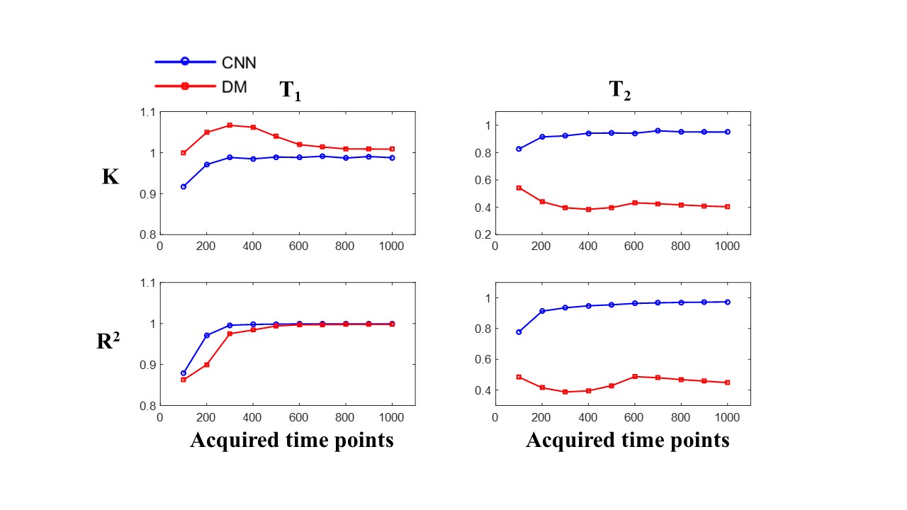
CNN is superior to DM in both T1 and T2 prediction for all tested numbers of time points (Fig. 4). The advantage of CNN is obvious in T2 prediction. In T1 prediction, the advantage is noticeable when much less signal evolutions are acquired (R2: N = 100, 0.879 vs. 0.863; N = 200, 0.971 vs. 0.899; N = 300, 0.996 vs. 0.975). Compared to DM with N = 1000, the reconstruction fidelity of CNN with N = 300 (Fig. 3) is much higher in terms of T2 (K: 0.923 vs. 0.404; R2: 0.935 vs. 0.449), and very similar in terms of T1 (K: 0.988 vs. 1.008; R2: 0.996 vs. 0.998).Discussion and Conclusion
In this study, CNN can achieve accurate prediction of parameters with less signal evolutions acquired, which proves that CNN can be used to accelerate the MRF acquisition. The results also show that CNN has a significant advantage in T2 prediction in comparison to DM, which may be caused by the relative large step of off-resonance frequency in DM and the strong generalization ability of CNN. Notably, the size of the training set for CNN is much smaller than that of the dictionary (100,000 vs. 785,700), further indicating that CNN is able to learn the signal evolution model of MRF. Thus, CNN is promising in the MRF reconstruction allowing shorter acquisition time and higher accuracy.Acknowledgements
NoneReferences
1. Ma, D., Gulani, V., Seiberlich, N., Liu, K., Sunshine, J. L., Duerk, J. L., & Griswold, M. A. (2013). Magnetic resonance fingerprinting. Nature, 495(7440), 187-192.
2. LeCun, Y., Boser, B. E., Denker, J. S., Henderson, D., Howard, R. E., Hubbard, W. E., & Jackel, L. D. (1990). Handwritten digit recognition with a back-propagation network. In Advances in neural information processing systems (pp. 396-404).
3. Kingma, D., & Ba, J. (2014). Adam: A method for stochastic optimization. arXiv preprint arXiv:1412.6980.
4. Srivastava, N., Hinton, G. E., Krizhevsky, A., Sutskever, I., & Salakhutdinov, R. (2014). Dropout: a simple way to prevent neural networks from overfitting. Journal of machine learning research, 15(1), 1929-1958.
5. Abadi, M., Agarwal, A., Barham, P., Brevdo, E., Chen, Z., Citro, C., ... & Ghemawat, S. (2016). Tensorflow: Large-scale machine learning on heterogeneous distributed systems. arXiv preprint arXiv:1603.04467.
Figures
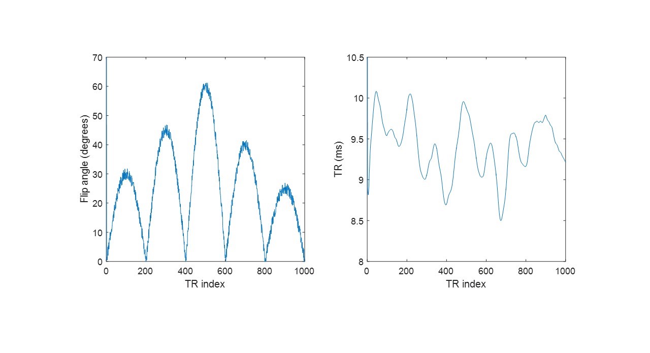
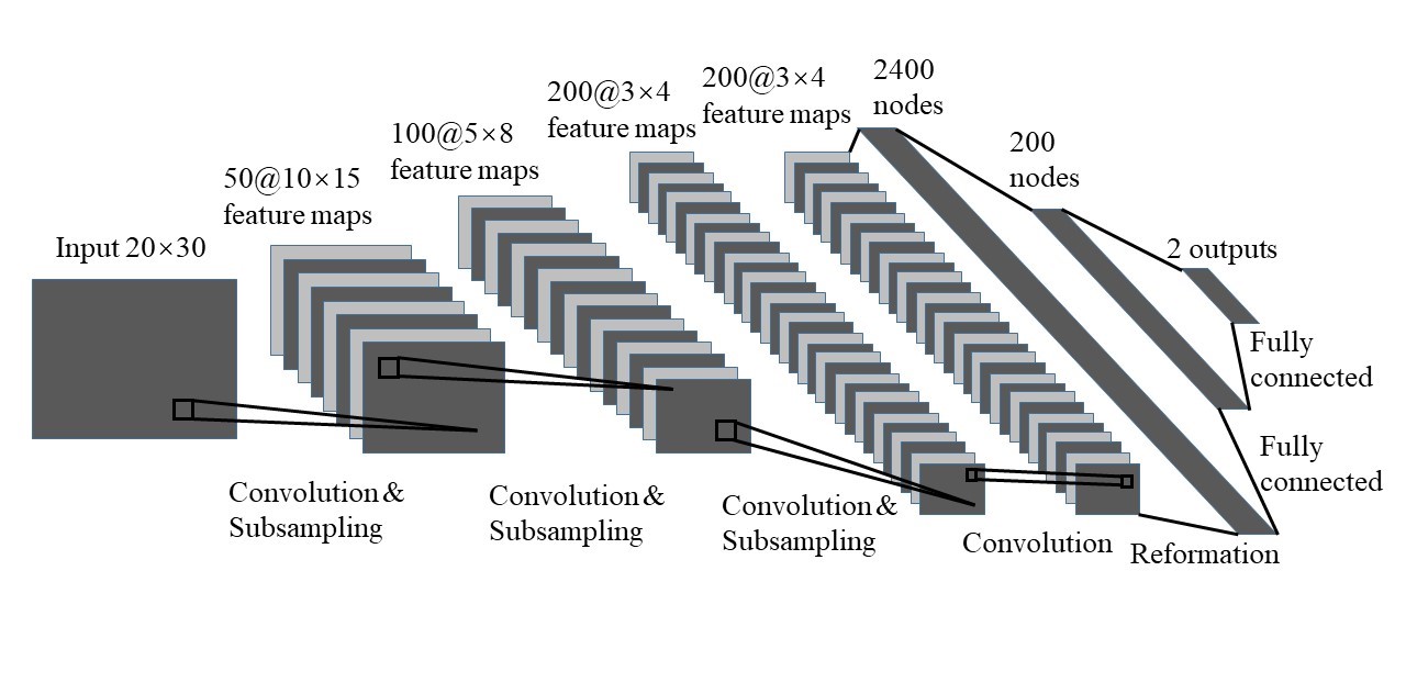
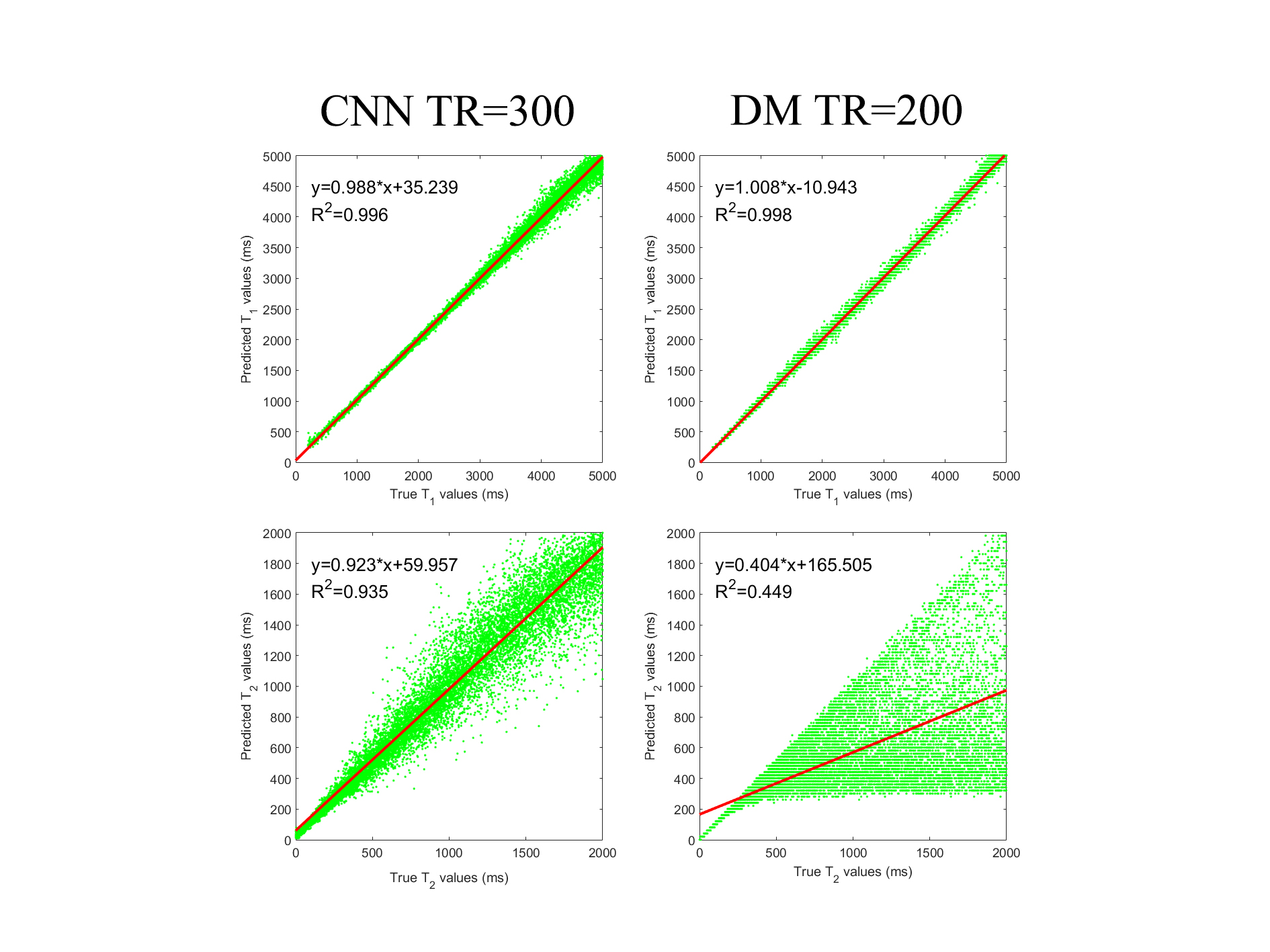
Figure 3. Linear regression of the predicted parameters with respect to the true values. The red line is the linear regression function with its formula on the top left corner. The left two images are acquired by CNN with N = 300. The right two images are acquired by DM with N = 1000.