4258
Hybrid-State Free Precession for Measuring Magnetic Resonance Relaxation Times1Bernard and Irene Schwartz Center for Biomedical Imaging, Dept. of Radiology, New York University School of Medicine, New York, NY, United States, 2Center for Advanced Imaging Innovation and Research (CAI2R), Dept. of Radiology, New York University School of Medicine, New York, NY, United States, 3Sackler Institute of Graduate Biomedical Sciences, New York University School of Medicine, New York, NY, United States
Synopsis
This work analyzes the spin physics in steady-state free precession sequences modified to smoothly vary sequence parameters, as suggested in MR Fingerprinting. We arrive at the conclusion that a transient state develops only in one direction, while the magnetization in the other two dimensions transitions adiabatically between steady states. We provide solutions of the Bloch Equations for this hybrid state and demonstrate the superior T1- and T2-encoding performance of the hybrid state compared to the steady state.
Introduction
The original MR-Fingerprinting1 (MRF) implementation was based on a balanced-SSFP sequence modified to employ varying flip angles. Recent work2,3 indicates that spherical coordinates allow for a compact description of relaxation processes in such sequences. Here, we provide a solution of the Bloch Equations in spherical coordinates. A comprehensive analysis of the solution reveals that the spin dynamics can be separated into a transient-state component and two components that adiabatically transition between steady states, which inspires the term "balanced hybrid-state free precession" (bHSFP). Numerical optimizations demonstrate the superior $$$T_{1,2}$$$-encoding power of the hybrid state compared to the steady state.
Theory
By applying a first order Taylor expansion with respect to sequence parameters (such as flip-angle, RF-phase, and $$$TR$$$) to the eigen-decomposition of the spin evolution matrix4,5, one can show that only the transient eigen-state parallel to the steady-state magnetization gets populated by smooth parameter variations. Spherical coordinates separate this transient component along the radial dimension $$$r$$$ from the adiabatic components along the direction of the phase $$$\varphi$$$ and the polar angle $$$\vartheta$$$. The latter two are given by the steady-state solution of the Bloch Equations6 and are approximated by$$\tan(\varphi-\frac{\phi}{2})=\frac{\cos\phi-\exp(-TR/T_2)}{\sin\phi}$$and$$\sin^2\vartheta=\frac{\sin^2\frac{\alpha}{2}}{\sin^2\frac{\phi}{2}\cdot\cos^2\frac{\alpha}{2}+\sin^2\frac{\alpha}{2}}$$anywhere except near the stop band. Here, $$$\alpha$$$ denotes the flip angle, $$$\phi$$$ the phase accumulated during one $$$TR$$$, and we define $$$\phi=\pi$$$ as on-resonance. Given these adiabatic transitions, the Bloch Equation along the radial direction is uncoupled and is solved by$$r(t)=a(t)\cdot\left(r_0+\frac{1}{T_1}\int_{0}^{t}\frac{\cos\vartheta(\tau)}{a(\tau)}d\tau\right)$$with$$a(\tau)=\exp\left(-\int_{0}^{\tau}\frac{\sin^2\vartheta(\kappa)}{T_2}+\frac{\cos^2\vartheta(\kappa)}{T_1}d\kappa\right),$$in which we assumed departure from $$$r_0$$$, and $$$t$$$ denotes time. Note that neither $$$\vartheta$$$, nor $$$r$$$ depend on $$$TR$$$, given $$$TR\ll\{T_1,T_2\}$$$.
Instead of an initial magnetization, we can also assume periodic or anti-periodic boundary conditions defined by $$$r(0)=\pm{r}(TC)$$$, where $$$TC$$$ denotes the duration of one cycle of the experiment. In this case, the radial Bloch Equation is solved by $$r(t)=\frac{a(t)}{T_1}\cdot\left(\int_{0}^{t}\frac{\cos\vartheta(\tau)}{a(\tau)}d\tau-\frac{a(TC)}{a(TC)\mp1}\int_{0}^{TC}\frac{\cos\vartheta(\tau)}{a(\tau)}d\tau\right).$$
Methods
On the search for the most efficient bHSFP sequence, we optimize the $$$\vartheta$$$-pattern. We employ the Broyden-Fletcher–Goldfarb-Shanno algorithm, and use the relative Cramer-Rao bound7-11 ($$$rCRB$$$), normalized by $$$TC$$$, as figure of merit. For comparison, optimizations were also performed for an inversion-recovery bSSFP sequence with a constant flip-angle12 and for a combination of spoiled gradient echo (SPGR) and bSSFP sequences in the steady state13.
In vivo measurements were performed with the anti-periodic bHSFP sequences, as well as with the optimized steady-state sequence, both with $$$TC = 3.8~\text{s}$$$. All experiments were performed on a 3T Prisma scanner (Siemens, Erlangen, Germany). Spatial encoding was performed with a sagittally oriented 3D stack-of-stars trajectory with golden angle increment14. The spatial resolution is $$$1~\text{mm}\times1~\text{mm}\times 2~\text{mm}$$$ at a FOV of $$$256~\text{mm}\times256~\text{mm}\times192~\text{mm}$$$. The total scan time was approximately $$$12.24~\text{min}$$$. Image reconstruction was performed with a low rank alternating direction method of multipliers approach15. $$$B_0$$$- and $$$B_1$$$-correction were performed on the basis of separate scans.
Results and Discussion
The optimized bHSFP sequences exhibit smooth $$$\vartheta$$$-patterns (Figure$$$~$$$1), and the spin dynamics, as described by the derived approximate solution of the Bloch Equations, shows good accordance with Bloch simulations anywhere apart from the vicinity of the stop-band (Figure$$$~$$$2).
When plotting the optimized $$$rCRB$$$ as a function of $$$TC$$$ (Figure$$$~$$$3), one can discriminate different aspects of underlying spin physics: All transient-state flavors result in a lower (i.e. better) $$$rCRB$$$ compared to the steady-state optimizations for scans longer than $$$2~\text{s}$$$. Note that the (anti-)periodic solutions represent transient state equivalents to the steady state in the sense that the RF-train can be repeated without waiting times, allowing for an efficient and flexible implementation of long RF-trains, e.g., for 3D imaging. Contrary to the periodic, the anti-periodic boundary condition allows for repeated visits of the southern hemisphere (Figure$$$~$$$1), which is reflected in a reduced $$$rCRB$$$ (green vs. black marks in Figure$$$~$$$3). The $$$rCRB$$$ difference between anti-periodic boundary condition and fully relaxed inversion-recovery design reflects the increased net-magnetization available at the start of the sequence (black vs. red marks). Further, comparing the IR-bSSFP to the IR-bHSFP optimization (brown vs. red marks) highlights the improvement in SNR due to a variable flip angles. These improvements are particularly pronounced at long $$$TC$$$ where the IR-bSSFP converges to a steady state. Figure$$$~$$$4 verifies that the $$$rCRB$$$ improvements span over large areas in $$$T_1$$$-$$$T_2$$$-space.
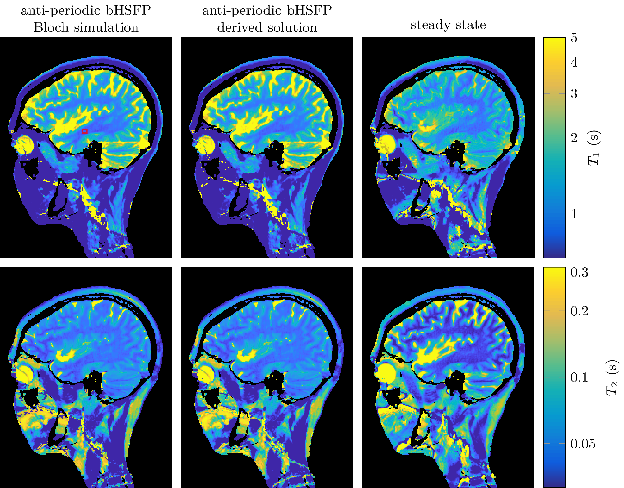
In vivo images reconstructed using full Bloch simulations and the proposed solution are in excellent agreement (Figure 5; $$$T_1=965\pm23~\text{ms}$$$ vs. $$$T_1=988\pm23~\text{ms}$$$ and $$$T_2=48.2\pm3.0~\text{ms}$$$ vs. $$$T_2=49.7\pm2.9~\text{ms}$$$). The superior SNR efficiency of the bHSFP patterns compared to an steady-state approach ($$$T_1=1035\pm72~\text{ms}$$$, $$$T_2=37.8\pm2.6~\text{ms}$$$) can also be seen in Figure$$$~$$$5. Systematic deviations can be noted, which we associate mainly with magnetization transfer16 and partial volume effects17, which are not yet considered in this work.
Conclusion
Slow sequence parameter variations result in a hybrid state, composed of transient- and steady-state components, which enables solving the Bloch Equations and provides insights on the spin dynamics.Acknowledgements
The authors would like to thank Steffen Glaser, Quentin Ansel and Dominique Sugny for fruitful discussions, and for giving insights into their optimal control implementation. The authors would also like to acknowledge Jeffrey Fessler and Gopal Nataraj discussions regarding the solution of the simplified Bloch Equation.
This work was supported by the research grants NIH/NIBIB R21 EB020096 and NIH/NIAMS R01 AR070297, and was performed under the rubric of the Center for Advanced Imaging Innovation and Research (CAI2R, www.cai2r.net), a NIBIB Biomedical Technology Resource Center (NIH P41 EB017183).
References
[1] Dan Ma, Vikas Gulani, Nicole Seiberlich, Kecheng Liu, Jeffrey L. Sunshine, Jeffrey L. Duerk, and Mark A. Griswold. Magnetic resonance fingerprinting. Nature, 495(7440):187–192, 2013.
[2] Jakob Assländer, Steffen J. Glaser, and Jürgen Hennig. Pseudo Steady-State Free Precession for MR-Fingerprinting. Magn. Reson. Med., 77(3):1151–1161, 2017.
[3] Jakob Assländer, Daniel K Sodickson, Riccardo Lattanzi, and Martijn A Cloos. Relaxation in Polar Coordinates: Analysis and Optimization of MR-Fingerprinting. In Proc. Intl. Soc. Mag. Reson. Med. 26, page 127, 2017.
[4] Brian A. Hargreaves, Shreyas S. Vasanawala, John M. Pauly, and Dwight G. Nishimura. Characterization and reduction of the transient response in steady-state MR imaging. Magn. Reson. Med., 46(1):149–158, 2001.
[5] Carl Ganter. Off-resonance effects in the transient response of SSFP sequences. Magn. Reson. Med., 52(2):368–375, 2004.
[6] Ray Freeman and H. D W Hill. Phase and intensity anomalies in Fourier transform NMR. J. Magn. Reson., 4(3):366–383, 1971.
[7] Calyampudi Radhakrishna Rao. Information and the Accuracy Attainable in the Estimation of Statistical Parameters. Bull. Calcutta Math. Soc., 37(3):81–91, 1945.
[8] Harald Cramér. Methods of mathematical statistics. Princeton University Press, Princeton, NJ, 1946.
[9] J.A. Jones, P. Hodgkinson, A.L. Barker, and P.J. Hore. Optimal Sampling Strategies for the Measurement of Spin–Spin Relaxation Times. J. Magn. Reson. Ser. B, 113(1):25–34, 1996.
[10] J A Jones. Optimal sampling strategies for the measurement of relaxation times in proteins. J. Magn. Reson., 126(126):283–286,1997.
[11] Bo Zhao, Justin P Haldar, Kawin Setsompop, and Lawrence L Wald. Optimal Experiment Design for Magnetic Resonance Fingerprinting. In Eng. Med. Biol. Soc. (EMBC), IEEE 38thAnnu. Int. Conf., number 1, pages 453–456, 2016.
[12] Peter Schmitt, Mark A Griswold, Peter M Jakob, Markus Kotas, Vikas Gulani, Michael Flentje, and Axel Haase. Inversion recovery TrueFISP: quantification of T1, T2, and spin density. Magn. Reson. Med., 51(4):661–667, 2004.
[13] Sean C L Deoni, Brian K. Rutt, and Terry M. Peters. Rapid combined T1 and T2 mapping using gradient recalled acquisition in the steady state. Magn. Reson. Med., 49(3):515–526, 2003.
[14] Stefanie Winkelmann, Tobias Schaeffter, Thomas Koehler, Holger Eggers, and Olaf Doessel. An Optimal Radial Profile Order Based on the Golden Ratio for Time-Resolved MRI. IEEE Trans. Med.Imaging, 26(1):68–76, 2007.
[15] Jakob Assländer, Martijn A Cloos, Florian Knoll, Daniel K Sodickson, Jürgen Hennig, and Riccardo Lattanzi. Low Rank Alternating Direction Method of Multipliers Reconstruction for MR Fingerprinting. Magn. Reson. Med., doi:10.1002/mrm.26639, 2017.
[16] Tom Hilbert, Tobias Kober, Tiejun Zhao, Kai Tobias Block, Zidan Yu, Jean-Philippe Thiran, Gunnar Krueger, Daniel K Sodickson, and Martijn Cloos. Mitigating the Effect of Magnetization Transfer in Magnetic Resonance Fingerprinting. In Proc. Intl.Soc. Mag. Reson. Med. 25, 2017.
[17] Debra McGivney, Anagha Deshmane, Yun Jiang, Dan Ma, and Mark A Griswold. The Partial Volume Problem in MR Fingerprinting from a Bayesian Perspective. In Proc. 24th Annu.Meet. ISMRM, page 435, 2016.
Figures
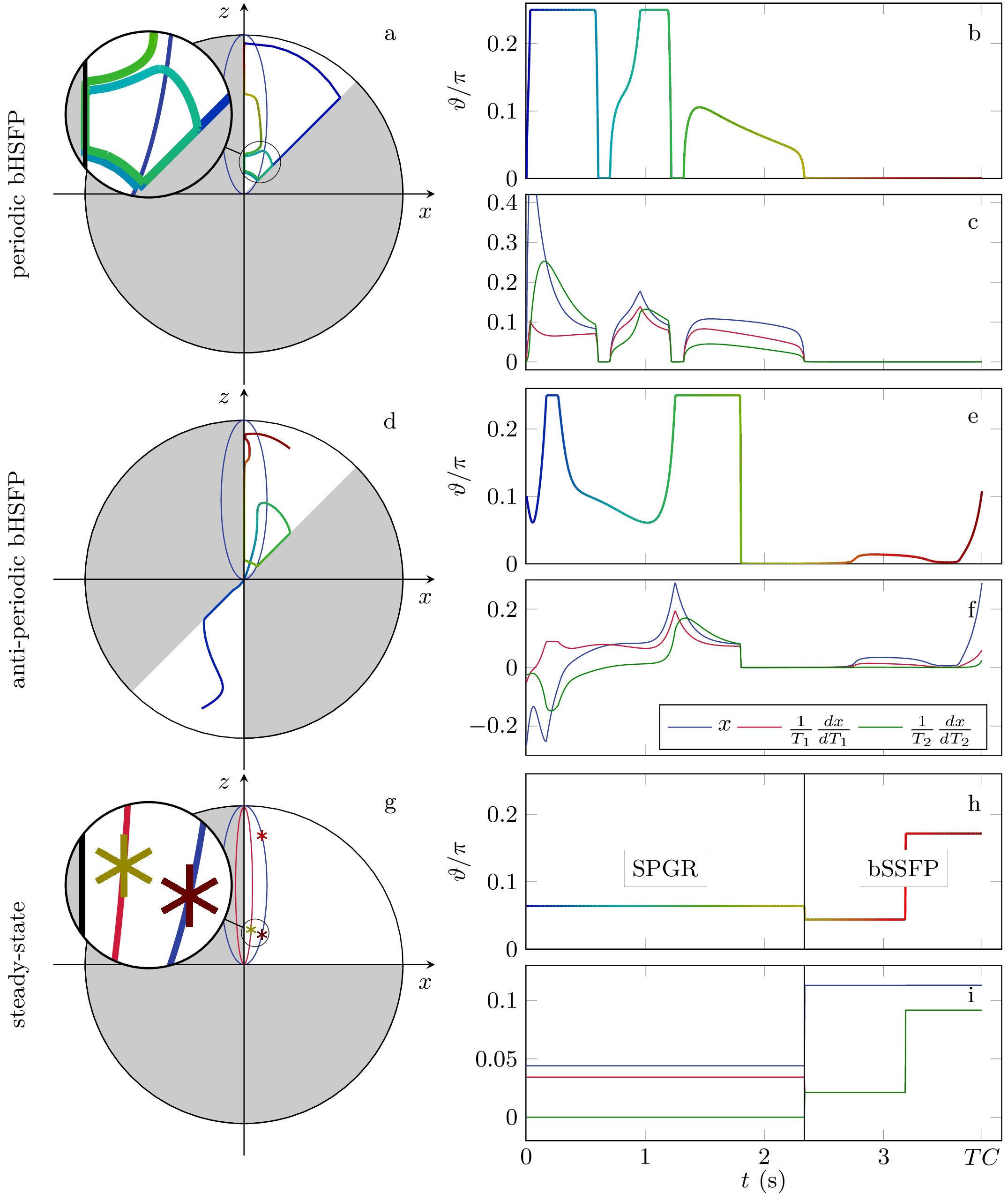
Figure 2: The derived solution of the Bloch Equations is verified against Bloch simulations at the example of the optimized anti-periodic pattern. In agreement with the approximate nature of the derivation, good accordance can be observed anywhere apart from the vicinity of the stop band. The gray areas indicate time points that were not acquired in the in vivo scan since the polar angle is close to zero.