Synopsis

It has been shown that the quantification of blood flow velocities through the use of bipolar gradients is possible within the MRF framework, called flow-MRF. In this work, we investigate four different flow encoding patterns for flow-MRF and analyze their impact on flow quantification. Finally we present an optimized pattern.

Purpose

Magnetic Resonance Fingerprinting (MRF) has emerged as an efficient technique for rapid quantification of relaxation parameters [1]. Recently, MRF was successfully used for quantification of blood flow velocities within vessels, termed flow-MRF [2], by modulating the first gradient moment (m₁) during the acquisition train.

In this work, we investigate four different m₁ patterns, analyze their impact on flow quantification, and present an optimized pattern. Changes in the velocity noise are quantified in phantom experiments and in-vivo applicability is shown.

Background

The first gradient moment is defined as: $$$m_1=\int{\gamma}tG(t)\mathrm{d}t$$$, where $$$\gamma$$$ is the gyromagnetic ratio and $$$G$$$ the gradient waveform. The phase accumulated by magnetization at spatial location $$$r$$$ and velocity $$$v$$$ while switching gradient $$$G$$$ is: $$$\varphi(r,v)=\gamma(m_0r+m_1v)$$$.

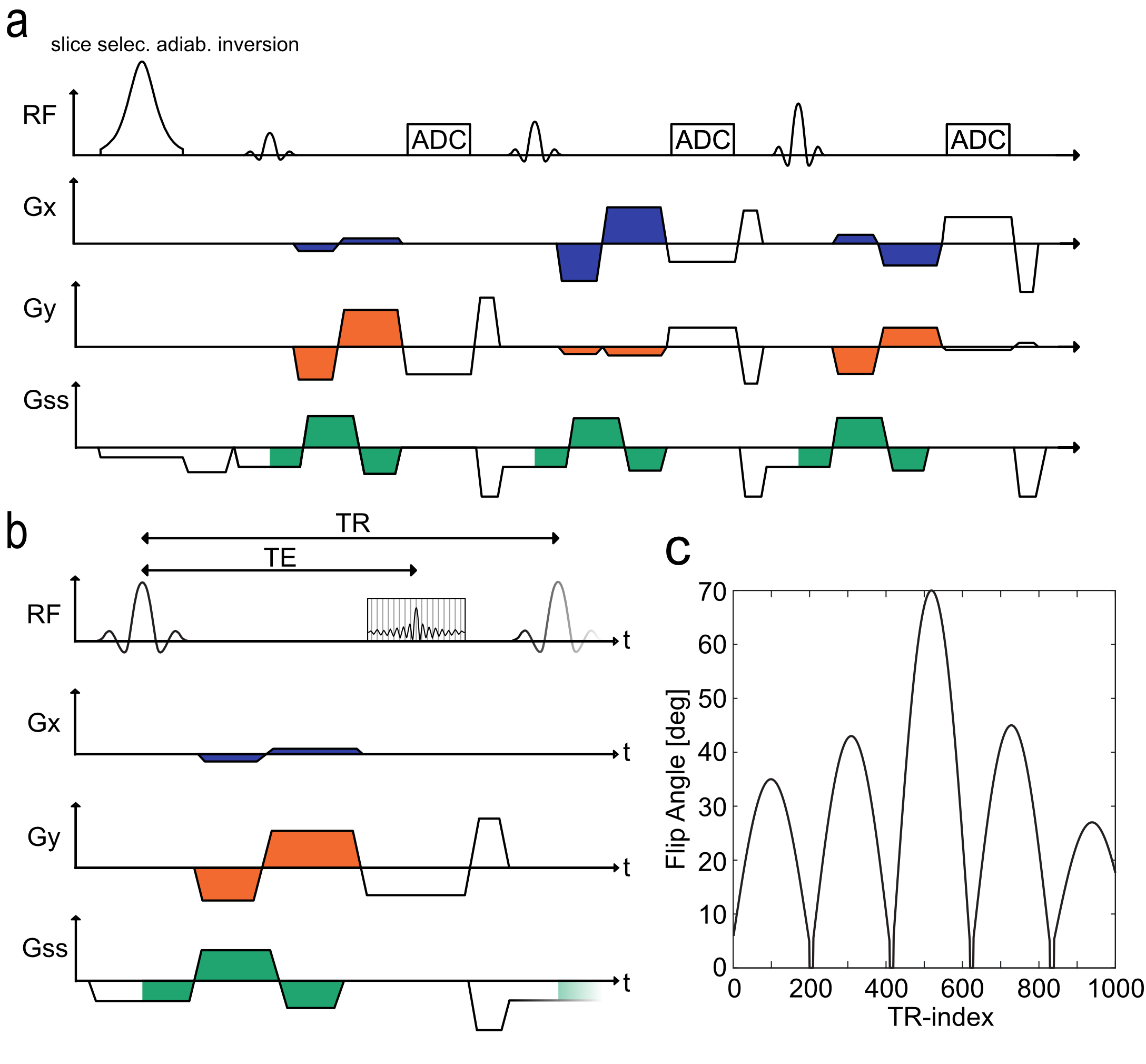
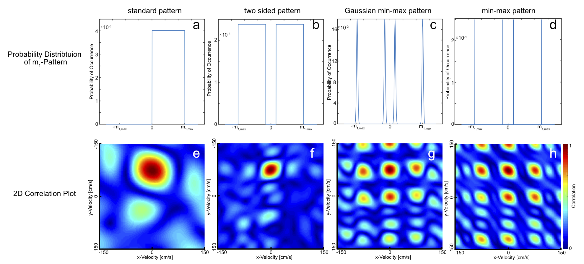
To achieve time-resolved, multi-directional velocity quantification in flow-MRF, bipolar gradients are integrated into a FISP-like radial MRF sequence (Fig.1), this allows the modulation of m₁ values throughout the acquisition train. The original flow-MRF sequence [2] used white noise distributions with minimum/maximum values $$$0/50\,\textstyle\frac{mT\cdot{ms}^2}{m}$$$ (Fig.2a).

Theoretically, a decrease in velocity noise inversely proportional to the maximum m₁ is expected. This is only valid if spatially and temporally constant velocity fields are present, characterized by a delta-peak velocity distribution. Both spatial and temporal gradients will be considered in the following evaluation of m₁ patterns. The impact of the maximum m₁ value (corresponding to a minimum velocity-encoding value $$$venc_{min}=\textstyle\frac{\pi}{\gamma{m_{1,max}}}$$$) will be investigated.

Methods

Four different patterns sampled randomly from the probability distributions illustrated in Fig.2a-d were investigated.

To evaluate each pattern's performance, a simulation closely modeling the MRF imaging process was used, taking into account relaxation, inflow of magnetization, gradient-induced dephasing, and undersampling effects. A numerical phantom was modeled according to an existing flow velocity phantom (Fig.4). The simulated resolution of 0.84$$$\times$$$0.84$$$\times$$$5mm$$$^3$$$ and the five radial projections per timeframe matched the conditions of subsequent phantom and in-vivo measurements.

For each pattern, three temporal velocity waveforms were simulated: i) constant velocity, ii) linearly ramped velocity, and iii) a realistic profile modeling flow in the femoral artery. Note that signal reduction due to intra-voxel dephasing originating from a range of different velocities within the voxels was considered during simulation. To determine a realistic pattern of intra-voxel velocities spatially resolved velocity distributions were measured by Fourier velocity-encoded imaging in the femoral artery [3]. Gaussian-shaped velocity peaks with FWHM of 15 cm/s were measured close to the vessel wall. Therefore, the three above-mentioned temporal velocity waveforms were investigated with two intra-voxel velocity distributions: a delta-peak and a Gaussian-shaped distribution with FWHM=15cm/s (Fig.3b).

Changes in velocity noise were quantified in phantom experiments with constant velocity. The standard deviation was calculated over 20 cardiac phases. The in-vivo applicability was demonstrated in the popliteal artery of a healthy volunteer.

Results

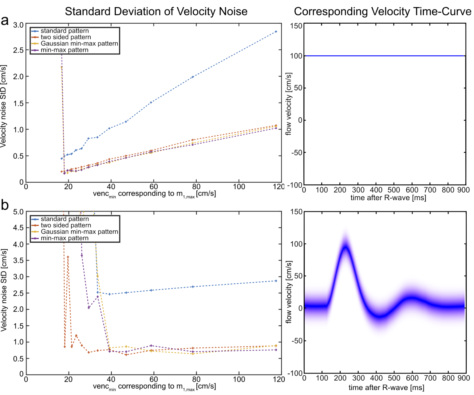
Fig.3 shows the velocity noise as a function of the maximum m₁ for the constant flow velocity with delta-distribution and the femoral artery flow profile with finite velocity spectrum. These two combinations represent the best and worst scenario, respectively, for flow quantification. All other combinations show similar behaviors and are not displayed. The constant velocity case demonstrates that all new m₁ encoding patterns achieve reductions in velocity noise by factors ≥2 compared to the standard pattern. The “min-max” pattern shows the overall lowest velocity noise for most m₁-values but the quantification becomes unstable at the highest m$$$_{1,max}$$$ of $$$70\,\textstyle\frac{mT\cdot{ms}^2}{m}\,(≙16.7\,\textstyle\frac{cm}{s}\,\,venc_{min})$$$. This is explained by Fig.2h, which shows the steepest gradient in the correlation around the global maximum, but strong local maxima nearby (up to 0.85) cause instability in the quantification. The femoral artery profile shows even higher noise reductions (factors ≥3) compared to standard encoding but only moderate dependency on the maximum m₁ value. For this profile the velocity quantification becomes unstable for all patterns if m$$$_{1,max}$$$ exceeds $$$50\,\textstyle\frac{mT\cdot{ms}^2}{m}$$$.

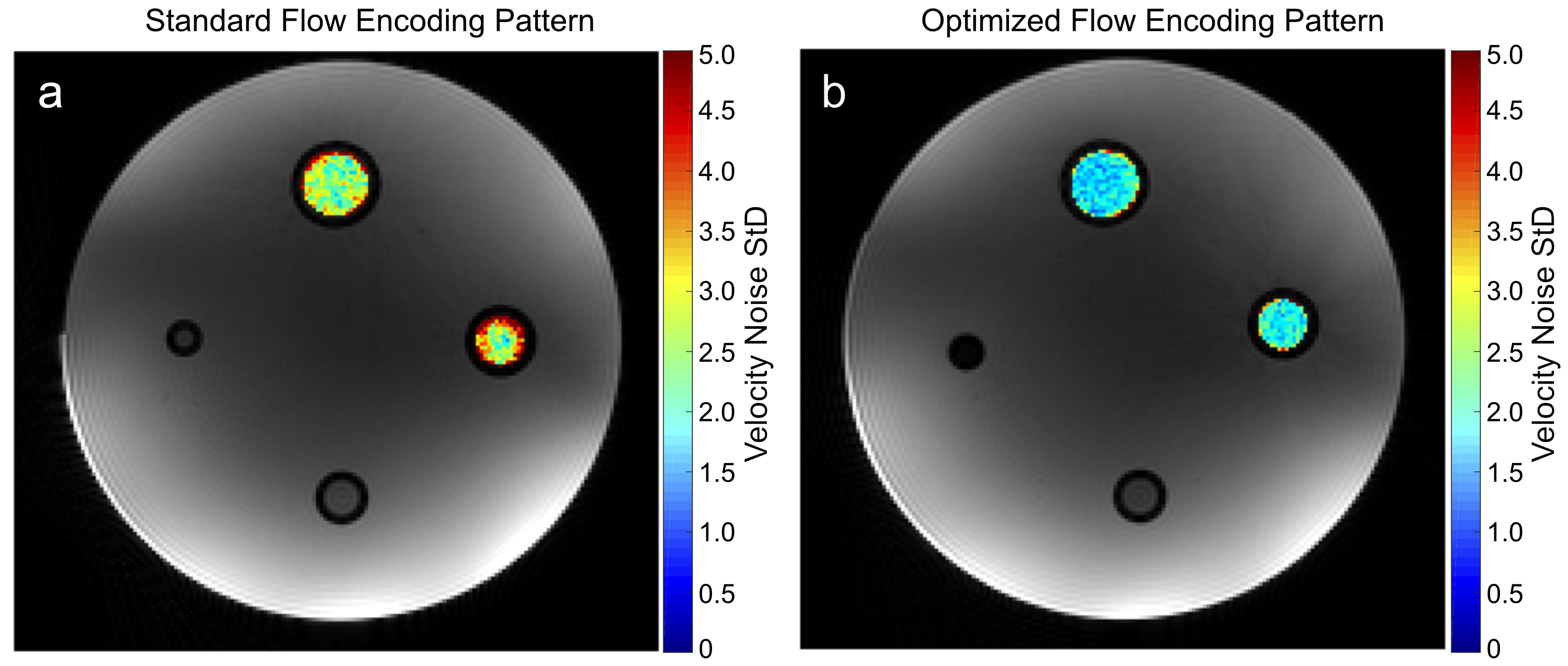
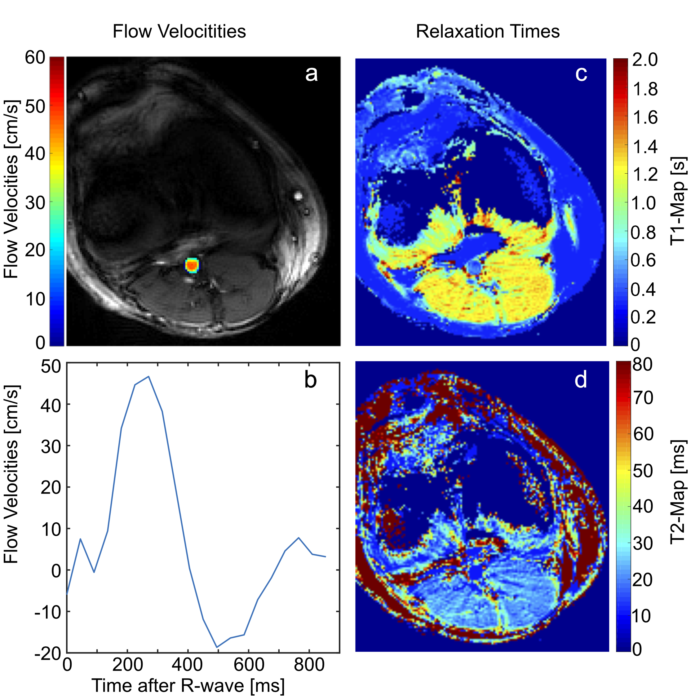
The “two sided” pattern with m$$$_{1,max}=30\,\textstyle\frac{mT\cdot{ms}^2}{m}\,(≙39.1\,\textstyle\frac{cm}{s}\,\,venc_{min})$$$ was identified as being optimal for phantom and in-vivo measurements. Velocity noise maps of the phantom experiment in Fig.4 reveal a 2.4-fold noise reduction on average. In-vivo results are presented in Fig.5, showing successful quantification of T₁ and T₂ as well as blood velocity.

Discussion and Conclusion

A 2.4-fold reduction in velocity noise was obtained using the optimized m₁ pattern for flow-MRF in the phantom, while robust velocity quantification in-vivo was maintained.

A conclusion of this study is that lower m₁ values might be preferable to achieve shorter echo times. This is reasonable because: 1) the strong temporal variations of the femoral artery profile show that noise is fairly unaffected by the maximum m₁ value and 2) dephasing of the velocity spectrum leads to signal losses. Furthermore, the potential for optimization in flow-MRF is demonstrated, and more rigorous studies will need to be performed to further increase the accuracy and efficiency of this method.

Acknowledgements

References

[1] Ma D, Gulani V, Seiberlich N, Liu K, Sunshine JL, Duerk JL, Griswold MA. Magnetic Resonance Fingerprinting. Nature 495, 187–192.

[2] Sebastian Flassbeck, Simon Schmidt, Mathies Breithaupt, Peter Bachert, Mark Ladd, Sebastian Schmitter. Quantification of Flow by Magnetic Resonance Fingerprinting. In Proceedings of the 25th Annual Meeting of the ISMRM, Honolulu, Hawaii, 2017. Abstract 0128.

[3] Moran, P. R. 1982. A flow velocity zeugmatographic interlace for NMR imaging in humans. Magn. Reson. Imaging 1: 197-203.