Synopsis

Spatially varying B₁ inhomogeneities and fat content are well known to be confounders of quantitative T₁ mapping that use multi flip angle techniques. Separate B₁ calibration maps can be acquired to correct flip angle errors cause by B₁ inhomogeneities, but this requires an additional acquisition. In this work we consider an alternative approach that acquires variable flip angles and variable repetition times, and simultaneously estimates B₁ inhomogeneity, T₁, fat-fraction and R₂*. The feasibility and noise performance of this approach are evaluated using theoretical Cramer-Rao Lower Bound analysis and simulations. Our results demonstrate that this approach is feasible, but suffers from relatively poor noise performance at typical acquisition parameters.

Introduction

T₁ mapping using the variable flip angle (VFA) method has multiple applications, particularly for body imaging where imaging speed and motion robustness are important (1,2). However, VFA is affected by two confounding factors: the presence of 1) fat and 2) B₁ inhomogeneities.

The presence of fat results confounds T₁ mapping of tissue parenchyma due to the short T₁ of fat signals. The presence of fat can be addressed through fat-water separated chemical shift encoded (CSE) techniques (3,4).

B₁ inhomogeneities result in spatially varying flip angle errors which, if uncorrected, lead to significant errors in VFA-based T₁ mapping (5,6). Previous B₁-corrected VFA methods use an external B₁ calibration acquisition to correct for spatially varying B₁ errors (6,7). In this work, we consider extending the CSE VFA method to jointly estimate fat-fraction and R₂* maps, as well as B₁, T_1W, and T_1F maps without an additional B₁ calibration scan. The purpose of this work is to propose and analyze a novel B₁- and fat-corrected CSE-MRI T₁ mapping method.

Theory

Transmitted flip angle (α_T) is related to prescribed flip angle (α_P) by the equation:

α_T=βα_P,

where β is the B₁ calibration coefficient. The spoiled gradient echo (SGRE) signal model (8-10) can be rewritten taking advantage of the relationship between transmitted flip angle, prescribed flip angle, and B₁ inhomogeneity as:

$$\pmb{S_n(\beta,\theta,\text{TR}_n,\alpha_{P_n},\text{TE}_n)=(\rho_W\frac{\text{Sin}\left(\beta\alpha_P\right)\left(1-e^{-\text{TR}\left/T_{1w}\right.}\right)}{1-\cos\left(\beta\alpha_P\right)e^{-\text{TR}\left/T_{1w}\right.}}+\rho_F\frac{\text{Sin}\left(\beta\alpha_P\right)\left(1-e^{-\text{TR}\left/T_{1F}\right.}\right)}{1-\cos\left(\beta\alpha_P\right)e^{-\text{TR}\left/T_{1F}\right.}}(\sum_{m=1}^Ma_me^{\text{j2$\pi\mathit{f}$}_m\text{TE}}))e^{j(\phi+\text{$\psi$TE})-R_2^*\text{TE}}}$$

Where θ=(ρ_W, ρ_F, T_1W, T_1F, Φ, ψ, R₂*) is the set of unknown parameters where ρ_W and ρ_F are the real-valued signals from water and fat, respectively, and T_1F and T_1W are their respective T₁ values; Φ is the initial phase for the fat and water signals (10); and ψ is the magnetic field inhomogeneity map. Additionally fat is jointly estimated, and therefore inherently corrected, by the inclusion of a 6-peak spectral model (11) of fat, where a_m and f_m are the corresponding relative amplitudes and frequencies of fat signals (8).

The subsequent sections examine the theoretical limitations of simultaneously estimating β as an unknown parameter from SGRE CSE-MRI data using variable flip angles and multiple TRs.

Methods

Analysis was designed for data acquired with 3 flip angles (α_P), 3 TRs, and 6 echo times per TR/α_P combination, resulting in 18 total acquisitions per reconstruction.

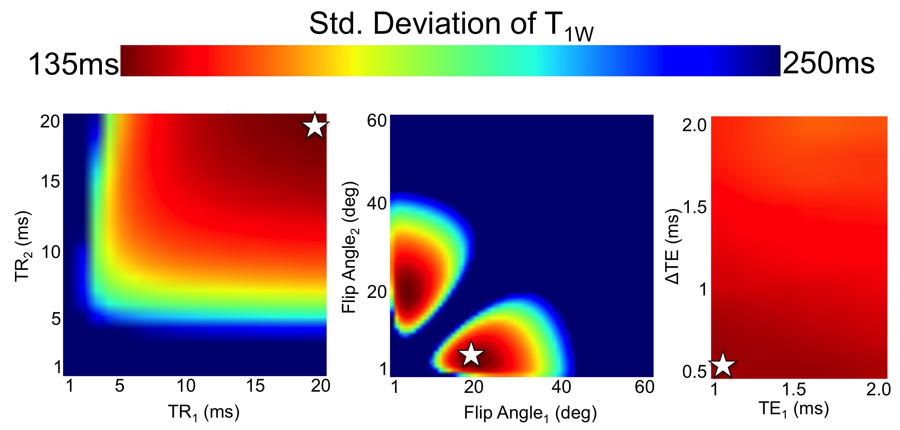
Optimization of Acquisition Parameters

A Cramer-Rao Lower Bound (CRLB) (12) was calculated for the 18-acquisition strategy described above. Results were used to determine the set of optimal acquisition parameters that would result in the smallest standard deviation of T_1W when β ≈1. Optimization was constrained to “reasonable” TR, TE, and flip angle (α_P) limits, such that TR<20ms, 1ms<TE₁<3ms, ΔTE >0.25ms, and 1^o< α_P<60^o. Additionally, SNR, defined here as mean(|S_n|)/σ, where σ=standard deviation of the noise), was set to a constant value of 60, which is an achievable value, eg: for 3D CSE-MRI of the liver (13).

Numerical Simulations

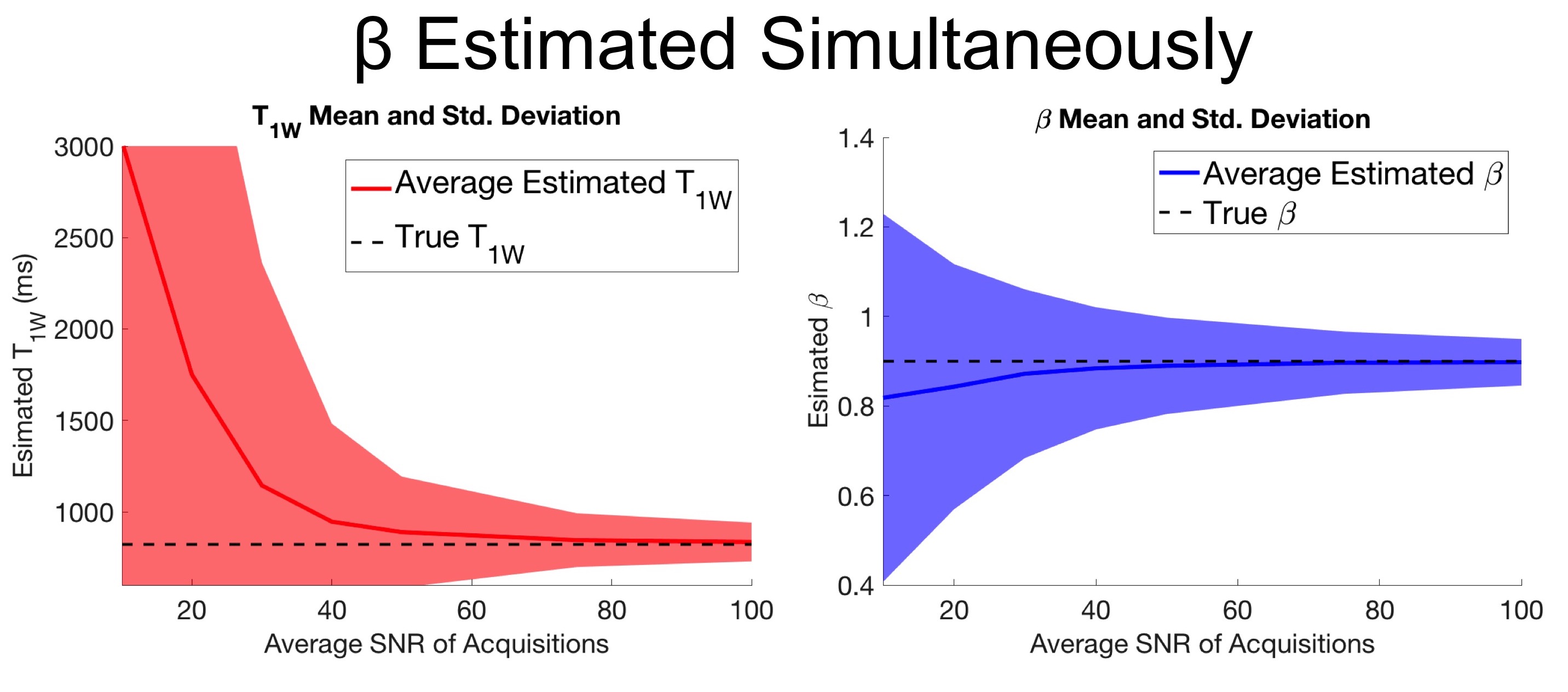
For a given set of unknown parameters including a small intentional B₁ inhomogeneity (β=0.9), T_1W=822ms, and PDFF=5% and acquisition parameters selected with CRLB analysis. 10,000 realizations of CSE-MRI were simulated with added zero-mean complex Gaussian noise. For each realization, a nonlinear least squares algorithm was used to estimate the set of unknown parameters, including β. This was repeated for SNR values over a range of 10-100.

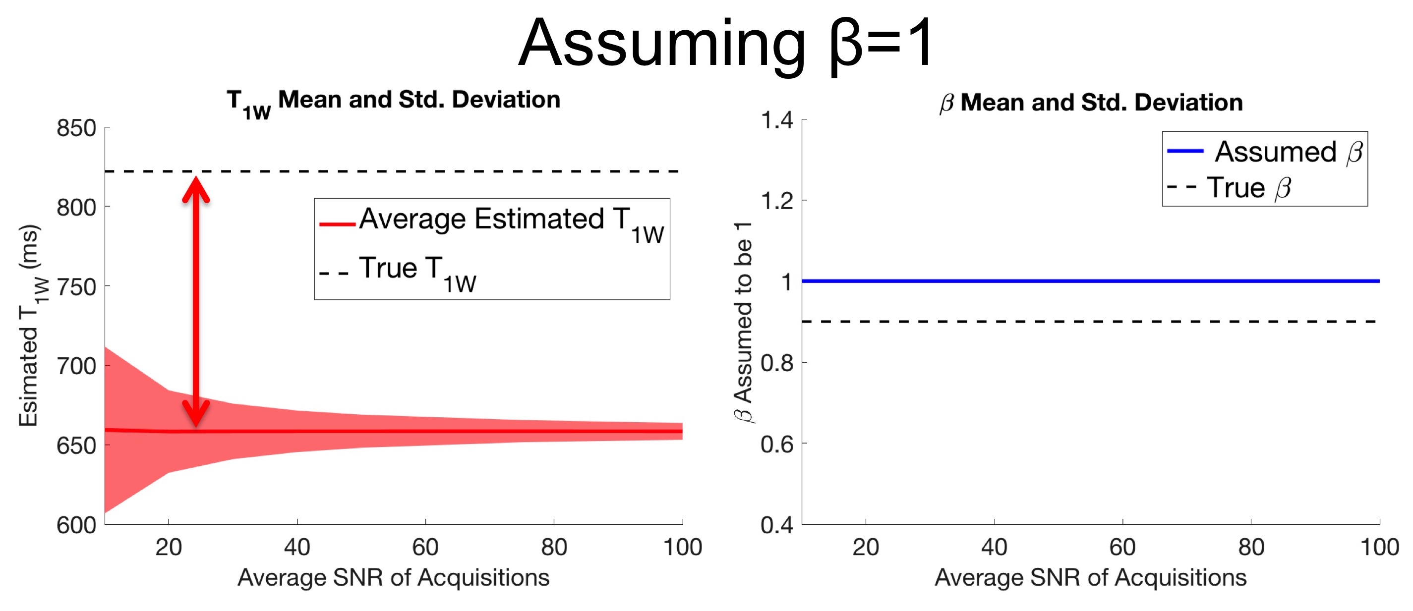
A second set of identical simulations was performed, except β was not estimated but was instead erroneously assumed to be 1.

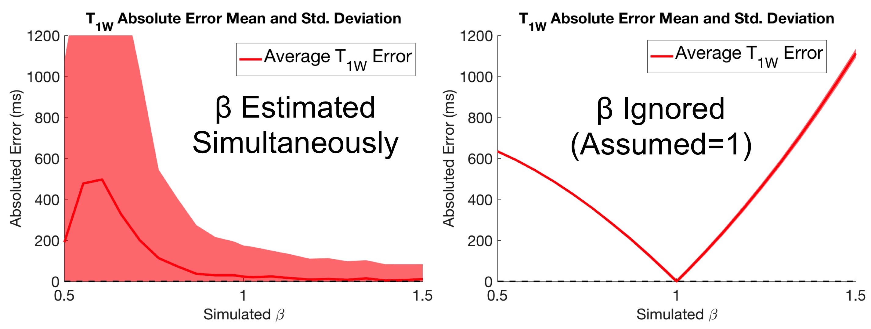
A final set of identical simulations was repeated, expect SNR was fixed at 60 and β was varied (0.5-1.5) for sets of 1,000 realizations.

Results

Optimization of Acquisition Parameters

CRLB analysis determined optimal α_P/TR pairs of 20^o/20ms, 5^o/20ms, and 60^o/20ms, with an initial echo time of TE₁=1.1ms and echo spacing ΔTE=0.3ms. Plots showing the CRLB optimization space are shown in Figure 1.

Numerical Simulations

Numerical simulations demonstrated convergence to an unbiased estimator for both T_1W and β when average SNR is approximately 80 when estimating β simultaneously. Results also demonstrated that relatively small flip angle errors cause large bias in T₁ estimation (Figures 2,3). Results also show β dependent bias in T₁ estimation for both simultaneously estimating and ignoring β methods (Figure 4).

Discussion

Acknowledgements

References

1. Brookes JA, Redpath TW, Gilbert FJ, Murray AD, Staff RT. Accuracy of T1 measurement in dynamic contrast-enhanced breast MRI using two- and three-dimensional variable flip angle fast low-angle shot. Journal of Magnetic Resonance Imaging 1999;9(2):163-171.

2. Deoni SC, Rutt BK, Peters TM. Rapid combined T1 and T2 mapping using gradient recalled acquisition in the steady state. Magn Reson Med 2003;49(3):515-526.

3. Liu CY, McKenzie CA, Yu H, Brittain JH, Reeder SB. Fat quantification with IDEAL gradient echo imaging: correction of bias from T(1) and noise. Magn Reson Med 2007;58(2):354-364.

4. Wang X, Hernando D, Wiens C, S. R. Fast T1 Correction for Fat Quantification Using a Dual-TR Chemical Shift Encoded MRI Acquisition. . 2017.

5. Deoni SC. Correction of main and transmit magnetic field (B0 and B1) inhomogeneity effects in multicomponent-driven equilibrium single-pulse observation of T1 and T2. Magn Reson Med 2011;65(4):1021-1035.

6. Cheng H-LM, Wright GA. Rapid high-resolution T1 mapping by variable flip angles: Accurate and precise measurements in the presence of radiofrequency field inhomogeneity. Magnetic Resonance in Medicine 2006;55(3):566-574.

7. Yarnykh VL. Actual flip-angle imaging in the pulsed steady state: a method for rapid three-dimensional mapping of the transmitted radiofrequency field. Magn Reson Med 2007;57(1):192-200.

8. Yu H, Shimakawa A, McKenzie CA, Brodsky E, Brittain JH, Reeder SB. Multiecho water-fat separation and simultaneous R2* estimation with multifrequency fat spectrum modeling. Magn Reson Med 2008;60(5):1122-1134.

9. Horng DE, Hernando D, Hines CD, Reeder SB. Comparison of R2* correction methods for accurate fat quantification in fatty liver. J Magn Reson Imaging 2013;37(2):414-422.

10. Bydder M, Yokoo T, Yu H, Carl M, Reeder SB, Sirlin CB. Constraining the initial phase in water–fat separation. Magnetic Resonance Imaging 2011;29(2):216-221.

11. Hamilton G, Yokoo T, Bydder M, Cruite I, Schroeder ME, Sirlin CB, Middleton MS. In vivo characterization of the liver fat (1)H MR spectrum. NMR Biomed 2011;24(7):784-790.

12. Scharf LL, Mcwhorter LT. Geometry of the Cramer-Rao Bound. Signal Process 1993;31(3):301-311.

13. Motosugi U, Hernando D, Wiens C, Bannas P, Reeder SB. High SNR Acquisitions Improve the Repeatability of Liver Fat Quantification Using Confounder-corrected Chemical Shift-encoded MR Imaging. Magn Reson Imaging 2017.