4235
AC magnetic sensing using the SIRS effect combined with bSSFP at ultra-low field1Radiology, Athinoula A. Martinos Center for Biomedical Imaging, Massachusetts General Hospital, Charlestown, MA, United States, 2Harvard Medical School, Boston, MA, United States, 3Physics, Harvard University, Cambridge, MA, United States
Synopsis
Direct detection of neuronal currents has long been a goal within MRI, with the aim of improving upon the spatial and temporal resolution of BOLD fMRI. So far, good results have been shown in phantoms but detection in vivo has proven difficult. A promising current detection technique is Stimulus-Induced Rotary Saturation (SIRS), but the BOLD signal can contaminate SIRS measurements, possibly explaining inconclusive in vivo results so far. A new sequence was developed and tested in an ultra-low-field (ULF) regime (6.5 mT) where paramagnetic effects such as BOLD are reduced and is more suited for SIRS measurements in vivo.
Purpose
To detect AC magnetic fields in an ultra-low-field (ULF) MRI system by creating a balanced Steady-State Free Precession (bSSFP) imaging technique that uses Stimulus-Induced Rotary Saturation (SIRS).Methods
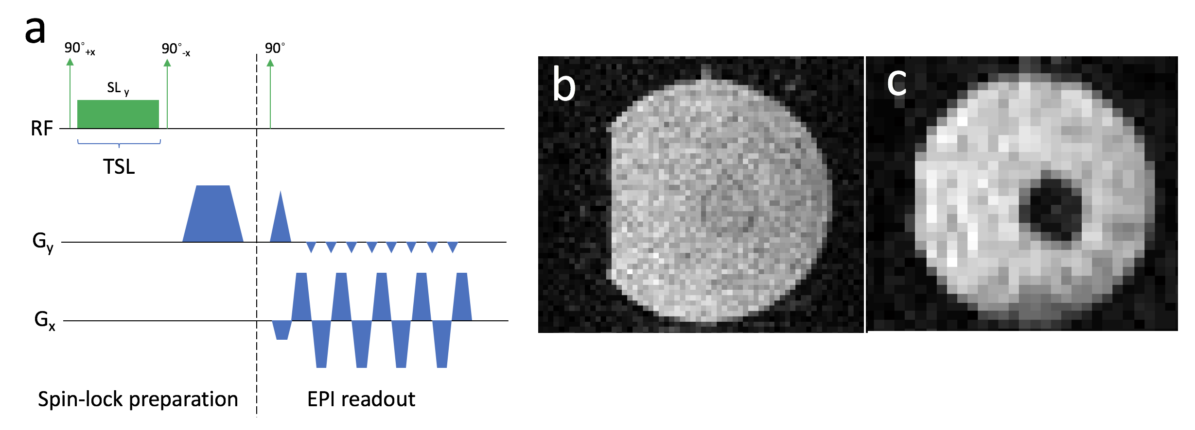
The SIRS sequence (Fig. 1) is a powerful method for measuring low-frequency magnetic stimuli with MRI1,2, but physiological effects such as BOLD make in vivo validation challenging. With the goal of investigating SIRS imaging at a low magnetic field with no BOLD contamination, a ULF 6.5 mT scanner with a maximum gradient amplitude of 1 mT/m was used. With these parameters, a normal SIRS scan would be slow and the small SIRS contrast hard to detect. The SNR efficiency of bSSFP results in a strong signal in reasonable scan times, particularly due to the near unity value of T2/T1 at such low magnetic fields, making it well suited for the ULF scanner3. Therefore, a new sequence, combining bSSFP with SIRS, was developed as shown in Fig. 2. The magnetization is flipped to the y-axis and a spin-lock pulse is applied, sensitizing the magnetization to the frequency γBSL. The magnetization will rotate by α=γBstimTSL away from the spin-lock axis in the doubly rotating frame, while also precessing by φ=γBSLTSL around BSL, thus lying on the cone shown in Fig. 2c. The magnetization is then rotated back to the normal rotating frame to enable signal readout and relaxation, before being flipped back in the next TR. Effectively, this will be a bSSFP sequence with a flip angle of α. While this angle will be small, the steady-state signal can be made large or small, since the bSSFP signal as a function of off-resonance or RF phase cycling gives high spikes spaced by 2π4.
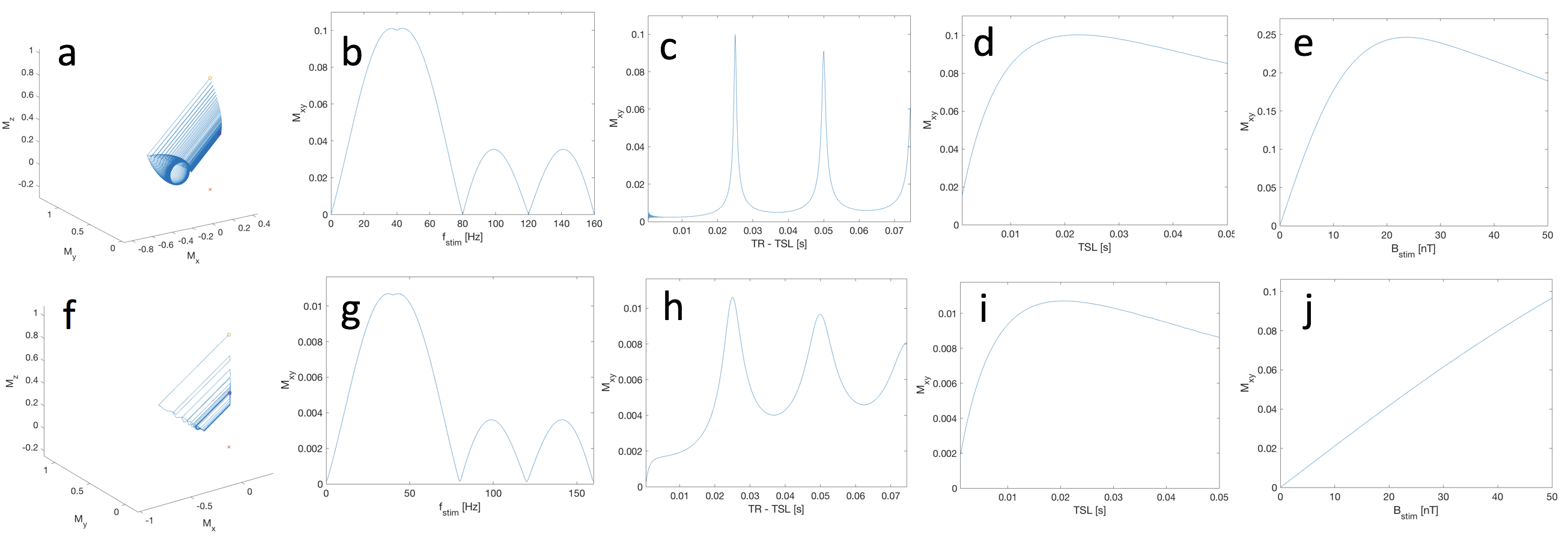
Bloch simulations of the sequence were performed in MATLAB (Fig. 3). The parameters were T1=630ms, T2=625ms, Bstim=5nT, fstim=40Hz, γBSL=40Hz, TSL=25ms, TR= 50ms. The parameters fstim, TR–TSL, TSL, and Bstim were then varied. The process was then repeated for T1=127ms and T2=76ms, the measured values for white matter at 6.5mT.
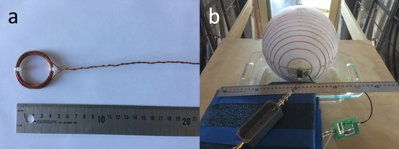
Then, a wire loop with a 4cm diameter and 10 turns was inserted into a phantom filled with CuSO4 solution (Fig. 4). A sinusoidal current was generated and passed through the loop. Experiments were performed with T1= 630ms, T2=625ms, Bstim=17nT, γBSL=100Hz, TSL=41ms, TR=55ms, and fstim= [90,95,97,100,103,105,110] Hz with a 32×32×19 imaging matrix, FOV= 28cm×21cm×20cm and 120 signal averages with a scan time of 33 min.
Results
The simulations showed the magnetization tracing a cone along the SL axis until settling on a circle in the steady-state. Varying the scan parameters showed quite similar behavior to bSSFP, such as a spike-like signal as a function of TR-TSL at small angles. This is because TR-TSL determines the relative phase difference between the stimulus wave and the magnetization between SL pulses, much like RF phase cycling in normal bSSFP. The simulations showed a roughly sinc shaped frequency response, as expected from the (rectangular) SL pulse. Since the linearly polarized stimulus field will have equal right-hand and left-hand circularly polarized components, it has a positive and negative frequency component in the doubly-rotating frame, whose responses add up.
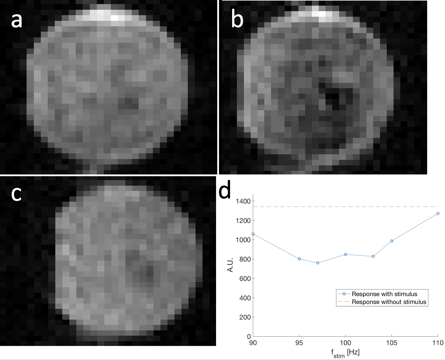
The phantom scans (Fig. 5) revealed a steady-state signal even without stimulus. This is likely due to off-resonance effects and was found to be minimized when the RF pulse was applied about 25 Hz off resonance. When the stimulus wave was turned on, it dominated this background signal and resulted in a net signal change of about 40%.
Discussion
Our observed signal change of 40% is quite large for a 17nT stimulus field, and carries promise of detecting much weaker stimuli in this system. This could eventually lead to the detection of fields from currents in neuronal bundles in the brain, expected to be around 0.1-1 nT5. The dark signal likely means we are between spikes in Fig. 3c. Future experiments will investigate other points along this curve.
The method described here not only allows SIRS imaging at our 6.5mT magnet, but also leverages several advantages of that system in addition to negligible BOLD contamination. Due to the operation at ULF, the repeated SL pulses throughout the scan do not raise SAR concerns. Furthermore, the scanner is very homogenous in absolute (Hz) terms, so achieving the desired point on the bSSFP curve (Fig. 3c) is more feasible than on standard clinical scanners.
Conclusion
A new bSSFP sequence using SIRS was developed, simulated, and used in phantom scans at a 6.5mT scanner. The simulations showed similar behavior to bSSFP and the phantom scans showed a 40% signal change with a stimulus field of 17nT.Acknowledgements
DARPA 2016D006054References
1: Witzel et al. Neuroimage 2008;42:1357-1365. 2: Jiang et al. MRM 2016;75:519–526. 3: Sarracanie et al. Nature Scientific Reports 2015;5:15177. 4: Carr. Phys Rev 1958;112:1693–1701. 5: Halpern-Manners et al. PNAS 2010;107:8519-8524.Figures