Synopsis

The goal of Contrast Source Inversion – Electrical PropertiesTomography is to iteratively reconstruct the conductivity and permittivity of tissue from $$$B_1^+$$$ field data. Up to now, this method has only been implemented in two dimensions. Here we demonstrate a proof-of-principle of a three-dimensional (3D) extension, thereby potentially turning CSI-EPT into a volumetric EPT technique. We present the basic 3D CSI-EPT equations, illustrate the performance of 3D CSI-EPT for realistic 3D body models, and show that accurate reconstructions are obtained even at tissue boundaries. The influence of the magnitude of the electric field on the reconstructions is also discussed.

Introduction

In Electrical Properties Tomography (EPT) we aim to reconstruct the conductivity $$$\sigma$$$ and permittivity $$$\epsilon$$$ of different tissues from transmit $$$B_1^+$$$ data collected within a region of interest. These electrical properties allow quantification of the specific absorption rate¹, can aid in the discrimination of cancerous and benign tissue² and can be used in hyperthermia treatment planning for the modeling of electromagnetic fields³.

EPT methods based on the homogeneous Helmholtz equation^1,4-9 show erroneous behavior at tissue transitions due to the assumed locally homogeneous media and are sensitive to noise since spatial differentiation operators act directly on the data. Contrast Source Inversion-Electrical Properties Tomography (CSI-EPT) is an iterative reconstruction method that circumvents these problems by making use of a global integral approach¹⁰. To date, CSI-EPT has only been implemented in two dimensions, while here we present a fully 3D implementation which takes all the EM field components into account.

Methods

In CSI-EPT, the body that occupies the domain $$$\mathbb{D}^{\text{obj}}$$$ is described by the dielectric contrast function $$$\chi=\epsilon_\text{r}(\mathbf{x})-1-\text{j}\sigma(\mathbf{x})/(\omega\epsilon_0)$$$, where $$$\sigma(\mathbf{x})$$$ and $$$\epsilon_\text{r}(\mathbf{x})$$$ are the conductivity and permittivity profiles, respectively. Furthermore, the contrast source $$$\mathbf{w}=\chi \mathbf{E}$$$ is introduced, with $$$\mathbf{E}$$$ the electric field. In CSI-EPT, both the unknowns $$$\mathbf{w}$$$ and $$$\chi$$$ are reconstructed by minimizing the objective function

$$F(\mathbf{w},\chi)=\frac{\|\mathbf{r}\|_{\text{obj}}^2}{\|\chi\mathbf{E}^\text{inc}\|_{\text{obj}}^2}+\frac{\|\rho\|_{\text{obj}}^2}{\|B_1^+\|_{\text{obj}}^2},$$

where the data residual

$$\rho=B_1^{+;\text{sc}}-\mathcal{G}_{\text{data}}\{\mathbf{w}\}$$

describes the mismatch between measured and modeled data, while

$$\mathbf{r}=\chi\mathbf{E}^\text{inc}-\mathbf{w}+\chi\mathcal{G}_{\text{obj}}\{\mathbf{w}\}$$

is the object residual, which describes the discrepancy in satisfying Maxwell’s equations. In the above equations,

$$\mathcal{G}_{\text{data}}\{\mathbf{w}\}(\mathbf{x})=\frac{\omega}{c_0^2}\tilde{\nabla}\cdot\int_{\mathbf{x}'\in\mathbb{D}^{\text{obj}}}G(\mathbf{x}-\mathbf{x}')\mathbf{w}(\mathbf{x}')\,\text{d}V$$

is the data operator that maps contrast sources to field data, while

$$\mathcal{G}_{\text{obj}}\{\mathbf{w}\}(\mathbf{x})=\left(\frac{\omega^2}{c_0^2}+\nabla\nabla\cdot\right)\int_{\mathbf{x}'\in\mathbb{D}^\text{obj}}G(\mathbf{x}-\mathbf{x}')\mathbf{w}(\mathbf{x}')\,\text{d}V$$

is the object operator mapping contrast sources to electric fields. Furthermore, $$$\tilde{\nabla}=-\frac{1}{2}(\mathbf{i}_x+\text{j}\mathbf{i}_y)\partial_z+\frac{1}{2}(\partial_x+\text{j}\partial_y)\mathbf{i}_z$$$ and $$$G$$$ is the scalar Green’s function of air.

Given initial guesses $$$\chi^{[0]}$$$ and $$$\mathbf{w}^{[0]}$$$, CSI-EPT first fixes the contrast function and updates $$$\mathbf{w}$$$ using a conjugate-gradient type update formula and subsequently updates $$$\chi$$$, while keeping the contrast source fixed¹⁰. This process is iteratively repeated until $$$F$$$ falls below an error tolerance, after which, at iteration $$$N$$$, the conductivity and permittivity profiles can be obtained as

$$\sigma=\text{Re}\left[\left(\chi^{[N]}+1\right)\text{j}\omega\epsilon_0\right]\quad\text{and}\quad\epsilon_\text{r}=\text{Re}\left[\left(\chi^{[N]}+1\right)\right].$$

Results & Discussion

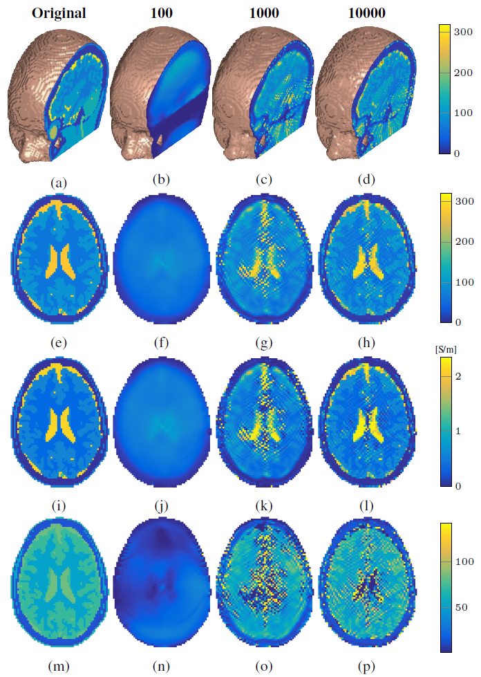
We consider the head of the 3D Ella model from the IT'IS Foundation¹¹ with an isotropic voxel size of 2.5 mm and simulate $$$B_1^+$$$ data from this region, generated by 16 $$$z$$$-directed dipoles each of length 30 cm, uniformly positioned on a circle around the head with a radius of 20 cm. The sources have a trapezoidal current distribution and operate in quadrature mode at 128 MHz (corresponding to 3T).

Fig. 1 shows the reconstruction of the head model, which has many small tissue interfaces and contains high conductivity and permittivity tissue. The 3D reconstruction after 100 iterations clearly shows that the center transversal slices are the most difficult to reconstruct. After 1000 iterations the tissue structure becomes visible, while after 10000 iterations we obtain a good overall agreement with the true model. Due to the increased complexity of the extension to 3D, the reconstruction of this fine-scaled head model takes about 20 hours with a Matlab implementation on a standard laptop. Computation times may be reduced by preconditioning techniques that reduce the number of CSI-EPT iterations.

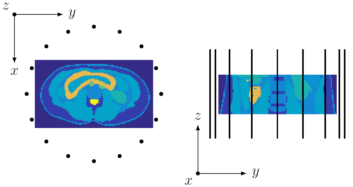
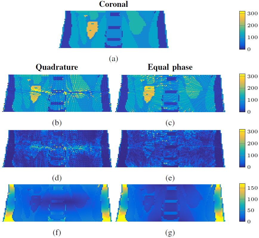
To study the influence of the electric field on the reconstructions, we consider the same antenna setup as before, but placed around the abdominal region of Ella (see Fig. 2) and we compare reconstructions obtained in quadrature and equal phase mode (no phase difference between sources). Even though equal phase would result in a nulling of the magnetic field, the reconstructions clearly show that regions with a relatively low electric field are the most difficult to reconstruct (see Fig. 3). Complementary antenna settings or active or passive $$$B_1$$$ shimming techniques can be used to improve reconstructions in these regions.

To investigate what tissue profiles CSI-EPT is able to retrieve, we have assumed noiseless $$$B_1^+$$$ data. In practice, both the amplitude and phase (collected in separate measurements) contain noise. Noise effects can be suppressed, however, by adding a regularization term to the objective function¹⁰. More critical is the presence of a receive phase component in the measured phase. Future work will therefore focus on developing a suitable signal model and objective function that takes this phase component into account.

Conclusion

Acknowledgements

References

1. Katscher U, Voigt T, Findeklee C, et al. Determination of electric conductivity and local SAR via B1 mapping. IEEE Trans Med Imag. 2009;28(9):1365–1374.

2. Kim S-Y, Shin J, Kim D-H, et al. Correlation between conductivity and prognostic factors in invasive breast cancer using magnetic resonance electric properties tomography (MREPT). Eur Radiol. 2016;26(7):2317–2326.

3. Balidemaj E, Kok H, Schooneveldt G, et al. Hyperthermia treatment planning for cervical cancer patients based on electrical conductivity tissue properties acquired in vivo with EPT at 3T MRI. Int J Hyperther. 2016;32(5):558–568.

4. Voigt T, Katscher U, and Doessel O. Quantitative conductivity and permittivity imaging of the human brain using electric properties tomography. Magn Reson Med. 2011;66(2):456–466.

5. van Lier A, Brunner D, Pruessmann K, et al. B1+ phase mapping at 7T and its application for in vivo electrical conductivity mapping. Magn Reson Med. 2012;67(2):552–561.

6. Sodickson D, Alon L, Deniz C, et al. Local maxwell tomography using transmit-receive coil arrays for contact-free mapping of tissue electrical properties and determination of absolute RF phase. inProc ISMRM, Melbourne, Vic., Australia,2012, p. 387.

7. Zhang X, van de Moortele P-F, Schmitter S, et al. Complex B1 mapping and electrical properties imaging of the human brain using a 16-channel transceiver coil at 7T. Magn Reson Med. 2013;69(5):1285–1296.

8. Liu J, Zhang X, van de Moortele P-F, et al. Determining electrical properties based on B1 fields measured in an MR scanner using a multi-channel transmit/receive coil: a general approach. Phys Med Biol. 2013;58(13):4395.

9. Marques J, Sodickson, Ipek O, et al. Single acquisition electrical property mapping based on relative coil sensitivities: a proof-of-concept demonstration. Magn Reson Med. 2015;74(1):185–195.

10. Balidemaj, C. A. T. van den Berg, J. Trinks, et al. CSI-EPT: a contrast source inversion approach for improved MRI-based electric properties tomography. IEEE Trans Med Imag. 2015;34(9):1788–1796.

11. Christ A, Kainz W, Hahn E, et al. The virtual family development of surface-based anatomical models of two adults and two children for dosimetric simulations. Phys Med Biol. 2010;55(2):23–38.