4219
Accelerated Imaging of Metallic Implants Using a 3D Convolutional Neural Network1Electrical Engineering, Stanford University, Stanford, CA, United States, 2Radiology, Stanford University, Stanford, CA, United States
Synopsis
Multi-Spectral Imaging (MSI) methods, such as SEMAC and MAVRIC-SL, resolve metal-induced field perturbations by applying additional encoding in the spectral dimension, at the cost of increased scan time. In this work, we introduce a 3D-CNN-based reconstruction to accelerate MSI utilizing spatial-spectral features of aliasing artifacts. We demonstrate in in vivo experiments that the proposed method can accelerate MAVRIC-SL acquisitions by a factor of 3 when used alone, and 17-25 when combined with parallel imaging and half-Fourier acquisition. The 3D-CNN showed significant improvement in image quality compared with parallel image and compressed sensing (PI&CS), with negligible additional computation time.
Purpose
Multi-Spectral Imaging (MSI) techniques, such as SEMAC1 and MAVRIC-SL2, resolve most metal-induced artifacts by acquiring separate 3D spatial encodings for multiple spectral bins (similar to slices), at the cost of increased scan time. Various methods have been explored to accelerate MSI by exploiting correlations between spectral bins3-5. Model-based reconstruction4 and RPCA5 explicitly or implicitly model spectral bin images as the same underlying magnetization modulated by different RF excitation profiles. They can provide around 20-fold acceleration when combined with parallel imaging (PI) and partial Fourier sampling (PF). However, they require long reconstruction times due to computationally expensive iterations.
Deep learning is an emerging technique in MRI reconstruction with negligible computation time compared to iterative methods6-9. In this work, we introduce a 3D convolutional neural network (3D-CNN) for accelerating MSI, which learns features of aliasing artifacts at different scales in spatial-spectral domain. We assess image quality in reader studies, comparing 3D-CNN output from retrospectively under-sampled data to the fully-sampled reference.
Methods
Reconstruction framework
The framework of the proposed 3D-CNN-based reconstruction is shown in Fig.1a. The under-sampled k-space data of each bin is first processed separately with PI & CS10. Next a 3D-CNN is used to remove residual aliasing artifacts and blurring in the initial bin images. The initial bin images are first sliced along the readout (x) direction, so that the input of the network has dimension [y, z, bin]. The output of the network is the residual image, which has the same dimension. The reconstructed bin images (initial + residual) are combined to form the final composite image.
Network architecture
A 3D U-Net11 architecture (Fig. 1b) with a total of 16 convolution layers is used for this study. The 2D U-Net12 has been popular in MRI reconstruction for its ability to learn features at different scales without losing high-spatial-frequency information7,8. Here the spectral dimension is treated equivalently to the spatial dimensions in convolutions, downscaling and upscaling operations. The spectral dimension can be preserved throughout the network by using 3D convolutions, but not 2D convolutions, as demonstrated in Fig.2.
Experiments
The 3D-CNN was trained and tested with MAVRIC-SL proton-density-weighted scans of 15 volunteers (8 for training, 7 for test) with total-hip-replacement implants. All scans were performed on GE 3T MRI systems with 24 spectral bins, 2x2 uniform under-sampling and half-Fourier acquisition. Other parameters include: 32-channel torso array, matrix size=384x256x(24-44), voxel size=1.0x1.6x4.0mm3. The images reconstructed by bin-by-bin PI&CS using all acquired data were used as the reference. Outer k-space was further under-sampled by 5 retrospectively with complementary Poisson-disc sampling13 (total R=17-25), and reconstructed by PI&CS and 3D-CNN. A total of 3072 training samples were used since y-z slices were reconstructed separately. Images were evaluated with normalized root-mean-square error (nRMSE), structural similarity index (SSIM), and scored by an experienced MSK radiologist using a 5-point scale (from 0 to 5: non-diagnostic; limited; diagnostic; good; excellent) in three categories: image sharpness, artifacts near metal and overall image quality.
Results
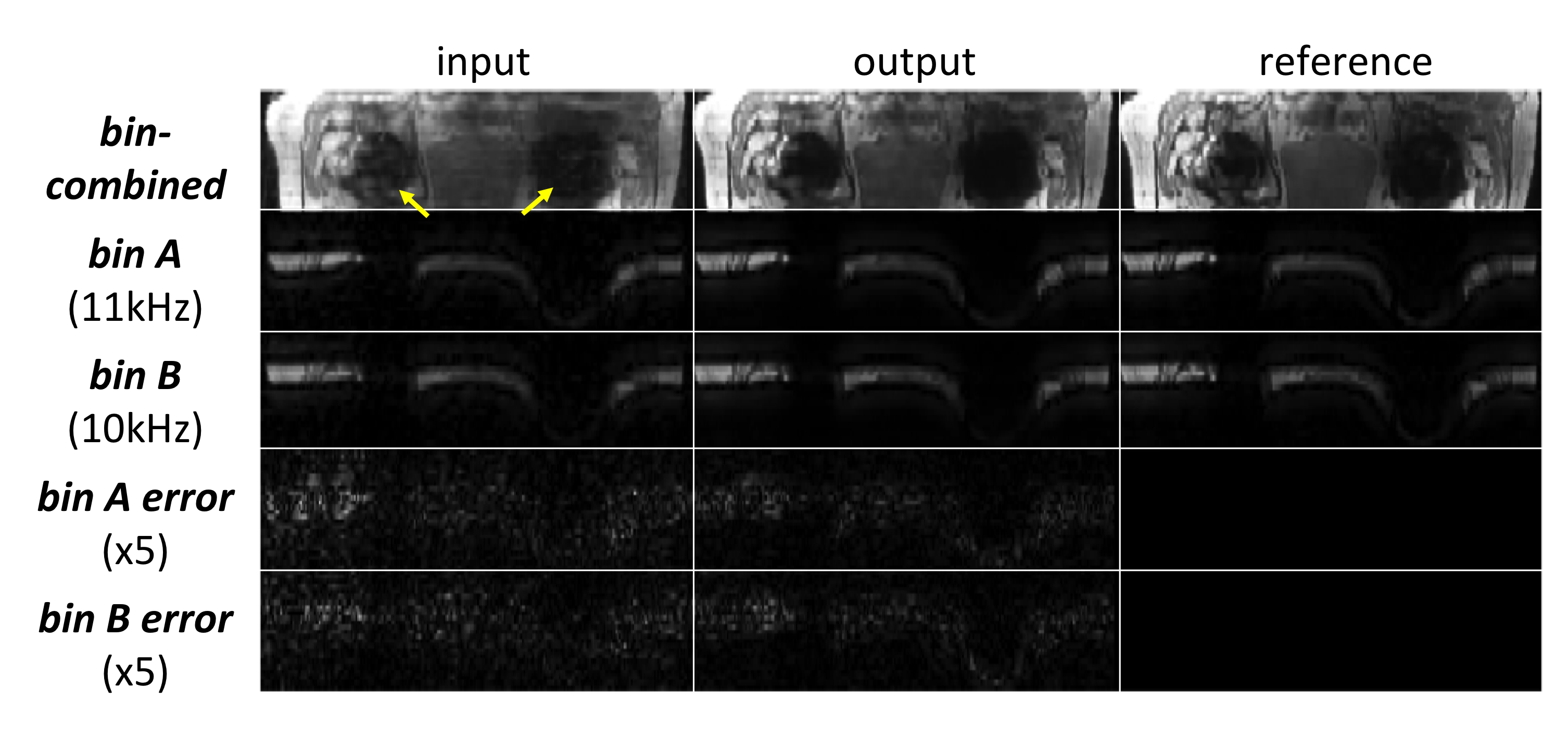
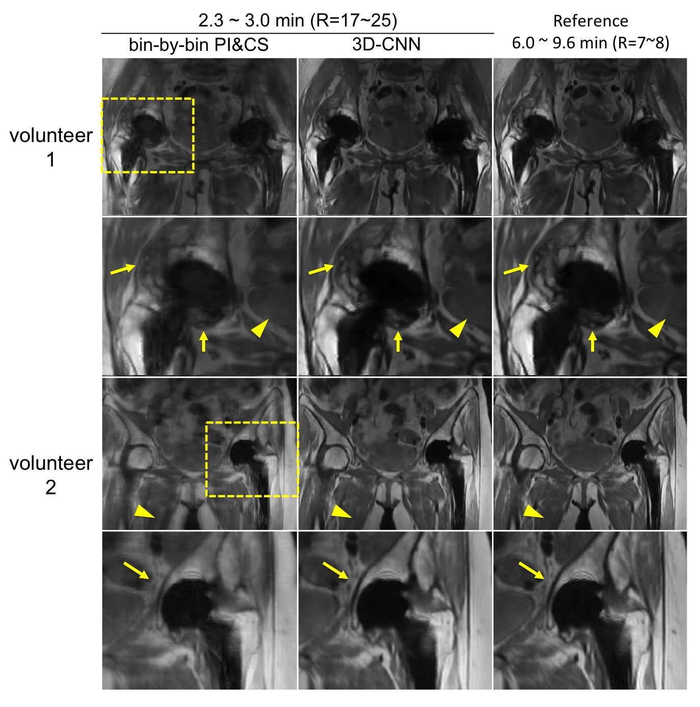
Fig.3 demonstrates the correlations between neighboring (and partly overlapping) spectral bins, and shows that 3D-CNN reduces error, especially in regions where each bin has low signals. Fig.4 compares the bin-combined images. 3D-CNN results showed improved image quality and sharpness over PI&CS across the field of view (FOV). For quantitative evaluation, the 3D-CNN reduced nRMSE from 11.7% to 9.0%, and increased SSIM from 0.81 to 0.86 on average. Radiologist scores (Fig.5) show a significant improvement in sharpness and overall image quality in 3D-CNN results compared to PI&CS (P<0.01), and no significant difference between 3D-CNN and the reference (P>0.05).Discussion
The 3D-CNN significantly improved the image quality of bin-by-bin PI&CS with negligible computation time (<10s with 1 GPU). The network learns aliasing artifacts effectively, because the encoder/decoder blocks can analyze and synthesize features at multiple spatial-spectral scales. We also experimented with a 2D U-Net architecture, which collapses the spectral dimension at the beginning, and the results were blurrier than 3D U-Net. The 3D U-Net architecture may be useful in other image reconstruction problems to utilize correlations in non-spatial dimensions, such as the temporal dimension.
The bin-by-bin initialization step integrates PI into the proposed reconstruction and reduced the dimension of the network by combining the coil images. Since this step is currently the bottleneck in terms of both computation and image quality, we will explore end-to-end deep learning in future work.
Conclusion
The proposed 3D-CNN-based reconstruction maintains high image quality at ~3x additional acceleration above partial Fourier and parallel imaging alone (~20x acceleration in total) with negligible additional computation time compared to PI&CS.Acknowledgements
NIH: R01 EB017739, R21 EB019723, P41 EB015891; research support from GE Healthcare.References
[1] Lu et al., MRM 62:66-76, 2009; [2] Koch et al., MRM 65:71-82, 2011; [3] den Harder et al., MRM 73: 233-243, 2015; [4] Shi et al., ISMRM 2016, p 47; [5] Levine et al., MRM DOI: 10.1002/mrm.26819, 2017; [6] Hammernik et al., ISMRM 2016: p.1088; [7] Han et al., ISMRM 2017: p. 690; [8] Lee et al., ISMRM 2017: p. 641; [9] Gong et al., ISMRM 2016: p. 5663; [10] Tamir et al., ISMRM Workshop on Data Sampling and Image Reconstruction, 2016; [11] Cicek et. al, MICCAI 2016: p. 424-432; [12] Ronneberger et. al, MICCAI 2015: p. 234-241; [13] Levine et. al, MRM 77:1774-1785, 2017.Figures