Synopsis

Multi-echo GRE sequence with bipolar readout gradients can reduce the achievable echo spacing compared to unipolar readout gradients for fat fraction (FF) quantification, and has higher acquisition efficiency. The eddy current induced phase (EC-phase) in bipolar sequence corrupts the phase consistency between the echoes, making it one of the confounding factors for the accurate fat quantification. In this study, we proposed an accurate EC-phase estimation method in bipolar acquisition sequence for FF quantification. The proposed method is validated through comparing the FF quantification from the EC-phase corrected bipolar data to the well-established unipolar acquisition through phantom experiments.

Introduction

Multi-echo GRE sequence with bipolar readout gradients can reduce the achievable echo spacing compared to unipolar readout gradients, and has higher acquisition efficiency in chemical shift-encoded imaging¹. The eddy current induced phase (EC-phase) in bipolar sequence is one of the confounding factors for fat quantification^2,3.

In this study, we proposed a method to estimate EC-phase in bipolar acquisition sequence for FF quantification. The proposed method is validated through comparing the FF from the EC-phase corrected bipolar data to the unipolar acquisition.

Materials and Methods

The signal can be represented as:

$$$ S_n=(W+F∑_{m=1}^Ma_mexp⁡(-i2πδ_mTE_n))∙exp⁡(-{TE}_n/{T_2^*})∙exp⁡(-i2πfTE_n) $$$(1)

where $$$a_m$$$ and $$$δ_m$$$ are the relative amplitude and chemical shift of m-th fat peak to the water, $$$∑_{m=1}^Ma_m=1$$$, single T2* model of fat and water is used in our study^{4, 5}.

With bipolar acquisition sequence, EC-phase is modulated to the even echoes as:

$$$S ̃_n=\begin{cases}S_n & n=1,3,5…\\S_n∙exp(iθ) & n=2,4,6…\end{cases}$$$(2)

where $$$S_n$$$ is defined as Eq.(1), and $$$θ$$$ is the EC-phase, which can be approximated by:

$$$θ=G_x x+G_y y+θ_0$$$(3)

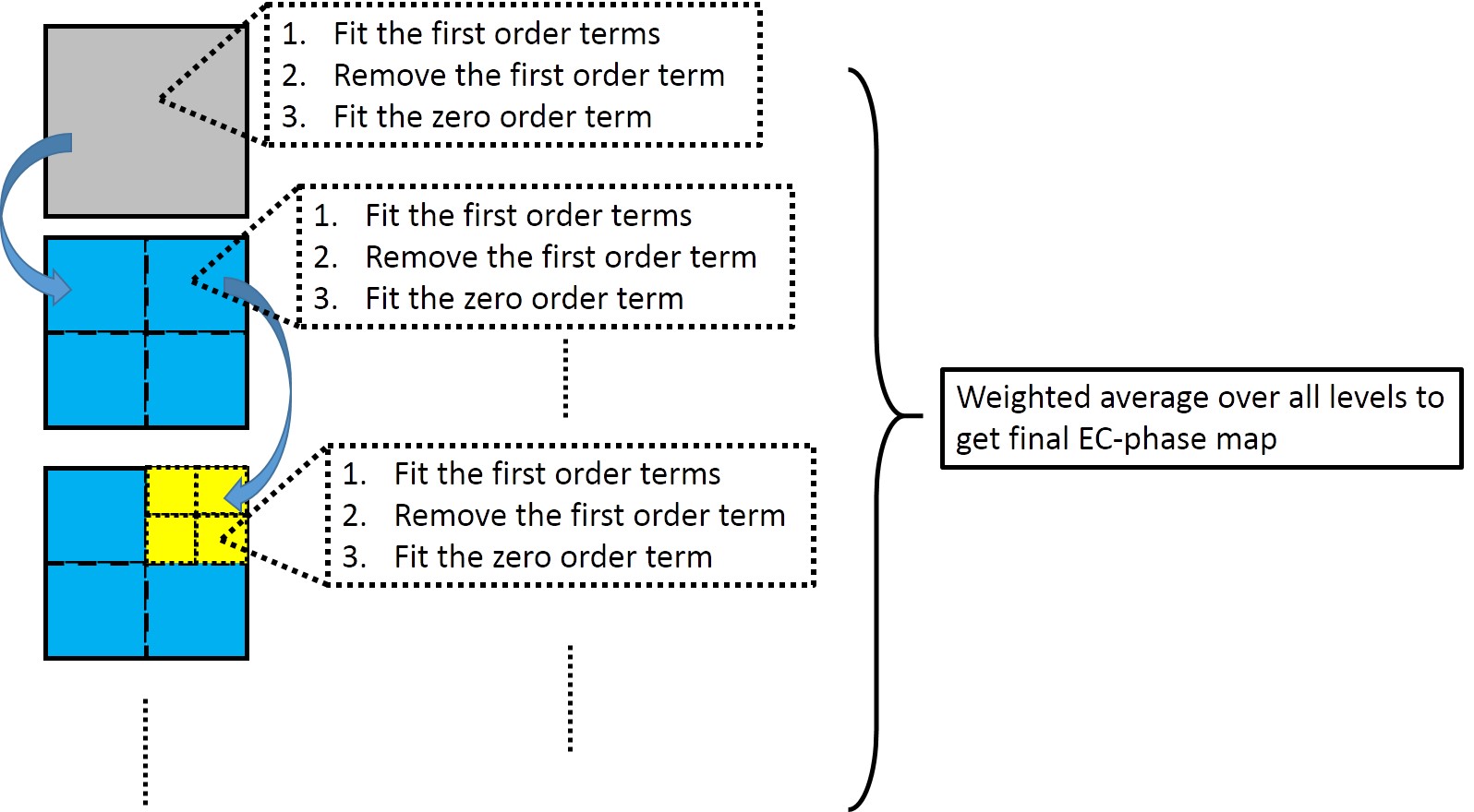
The proposed EC-phase estimation is shown in Figure 1.

Step1 (First order term):

For the pixel satisfying

$$$S_n (x,y,z)≈S_n (x-1,y,z) $$$(4)

define:

$$${DS}_n (x,y,z)=\frac{{S ̃_n (x,y,z)}}{{S ̃_n (x-1,y,z)}}=\frac{{S_n (x,y,z) exp⁡[i(1+(-1)^{(n-1)})/2\cdot(G_x x+θ_0 )]}}{S_n (x-1,y,z)exp⁡[i(1+(-1)^{(n-1)})/2\cdot(G_x (x-1)+θ_0 )]}≈exp[i(1+(-1)^{(n-1)})/2\cdot{G_x}] $$$(5)

Let:

$$$DX(x,y,z)=\frac{{DS}_2 (x,y,z)\cdot…\cdot{DS}_{2M} (x,y,z)}{{DS}_1 (x,y,z)\cdot…\cdot{DS}_{2M-1} (x,y,z)}=exp⁡(-i2MG_x ),2M<N$$$(6)

and $$$G_x$$$ can be fitted by:

$$$G_x=\frac{1}{2M}angle(\frac{1}{P}∑_pDX)$$$(7)

where, p is the index of those pixels satisfying Eq.(3). Similar operations can be done in y/z direction to obtain $$$G_y$$$ and $$$G_z$$$.

Step2 (Zero order term):

The first order term of phase error is removed from Eq. (3), and

$$$S ̃ ̃_n=\begin{cases}S_n & n=1,3,5…\\S_n∙exp(iθ_0) & n=2,4,6…\end{cases}$$$(8)

In pixels that contain only one species (water or fat), the signals become:

$$$S ̃ ̃_n=Wexp(-{TE}_n/{T_2^*})\cdot{exp(-i2πfTE_n)}\cdot{exp⁡(i(1+(-1)^N)θ_0/2)}$$$

or

$$$ S ̃ ̃_n=F∑_{m=1}^Ma_mexp⁡(-i2πδ_mTE_n )∙exp(-TE_n/{T_2^*} )∙exp(-i2πfTE_n)∙exp⁡(i(1+(-1)^N)θ_0/2)$$$(9)

To find pixels that contain only water or fat, one could either use magnitude fitting⁴, or complex fitting from even echoes to find where the FF is about 0 or 1.

As the equally-spaced TEs (six or more) are commonly used in the multi-echo GRE sequences for fat quantification, define

$$$ D(x,y,z)=\frac{S ̃ ̃_{2k+1}\cdot S ̃ ̃_{2k+1}}{S ̃ ̃_{2k}\cdot S ̃ ̃_{2k+2}},1≤2k<2k+2≤N $$$(10)

Terms that contain $$$TE_n$$$ are all canceled out in D, leaving

$$$D(x,y,z)=exp⁡(i2θ_0)$$$(11)

A practical solution of $$$θ_0$$$ is

$$$θ_0=\frac{1}{2}angle(\frac{1}{Q}∑_qD)$$$(12)

where q is the index of the pixels satisfying (9).

Phantom study

A series of fat containing water phantom with FF as 10%, 20%, 30%, 40%, 50% was built⁶. Along with a pure peanut oil phantom, the six phantoms were put in a tank filling with water. MR scans were conducted in a Siemens TIM Trio 3T system. 3D multi-echo gradient echo sequence was used for both unipolar/bipolar acquisitions with the following parameter: TR=20, imaging resolution = 2*2*3mm3, FA=3⁰. A unipolar readout dataset was acquired as reference. For both unipolar/bipolar acquisitions, the first TE was fixed to minimally allowed 1.78ms. For the bipolar acquisition, ΔTE=1.5/0.96ms were scanned. Imaging plane were firstly set in normal coronal orientation (Normal Slices), and then rotated 45⁰ in-plane for oblique acquisition (Oblique Slices). The phantoms were scanned for three times with the phantoms placed in the left, middle, and right side of the water tank. Temperature induced water frequency shift was corrected⁷.

The EC-phase removed data was processed by algorithm⁸ to get FF. Meanwhile, the accuracy of FF to the unipolar dataset was also compared with the EC-phase joint estimation method⁹.

Results

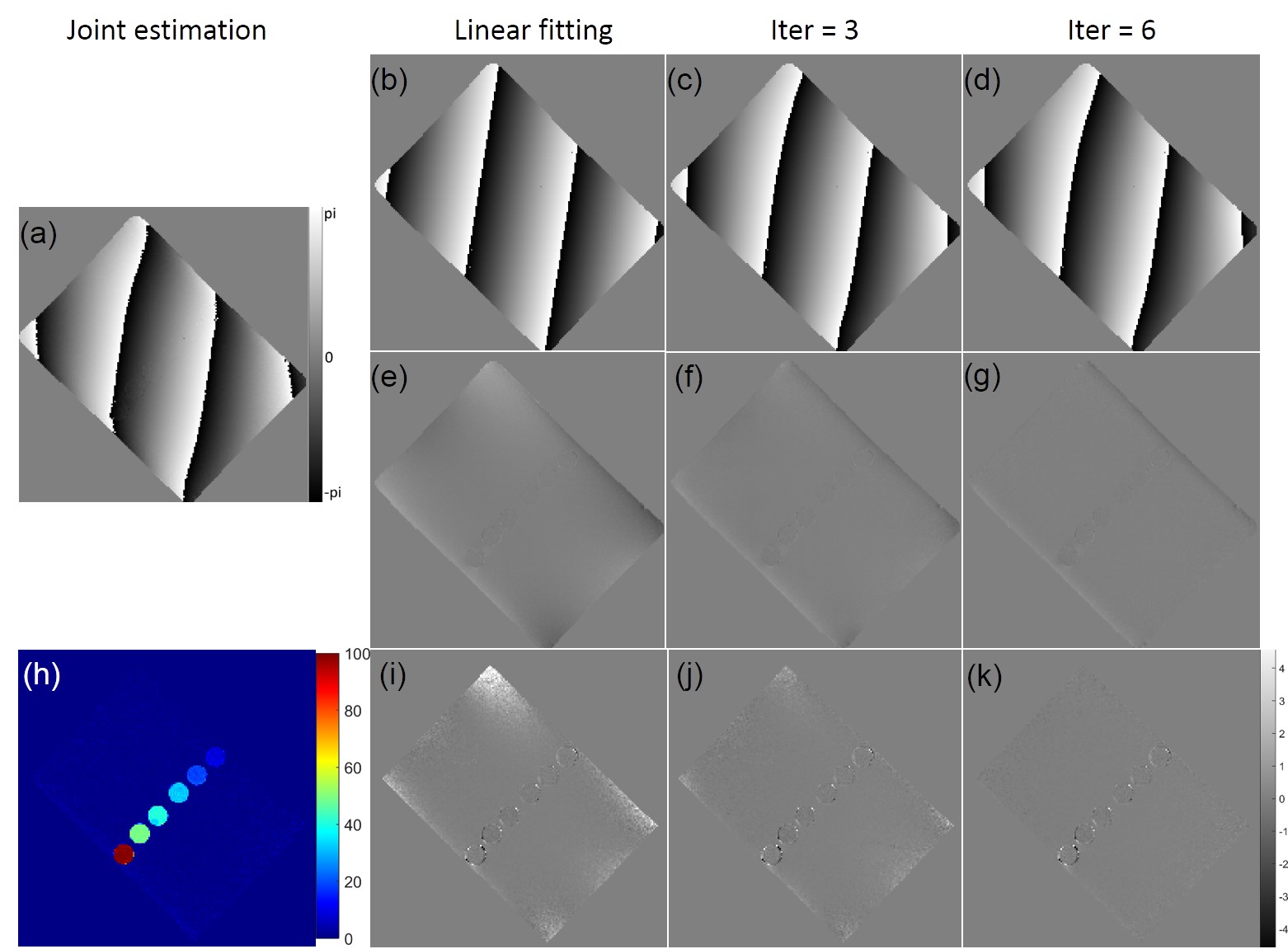
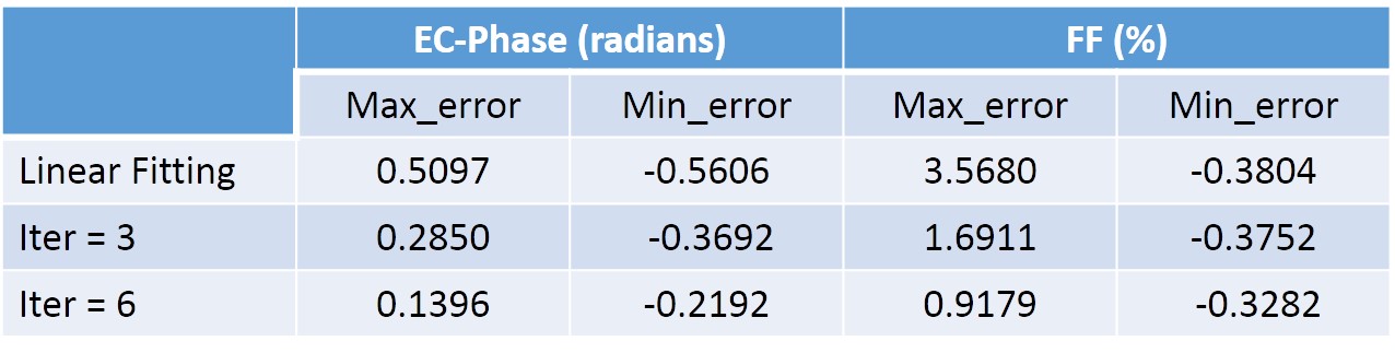
Figure 2 shows the EC-phase estimation results of the proposed method. Table 1 shows the EC-phase error and FF error. All results used the joint estimation method as reference.

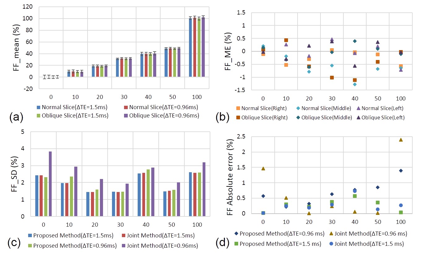
Figure 3 shows the phantom results. Comparing to the unipolar results, all tubes had similar FF whenever they were put in the right/middle/left side of water tank. The results were consistent between the datasets in Normal/Oblique slices with ΔTE=0.96/1.5ms. The precision of the joint method was poor especially in FF around 0 and 1 when ΔTE=0.96ms.

Discussions and Conclusions

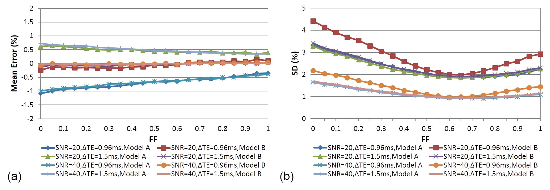
The phantom study shows the proposed EC-phase estimation method results in small FF error compared to the unipolar results, suggesting the EC-phase estimation error is rather limited. The phantom results can be also validated with the simulation shown in Figure 4. For ΔTE=0.96ms, the EC-phase joint estimation method has larger noise, especially for tubes with FF=0%, 10% and 100% (Figure 3c). As a result, the overall errors in these tubes are larger. For ΔTE=1.5ms, the mean and SD of FF error show no difference between the proposed method and the joint estimation method, suggesting EC-phase might be a redundant parameter at the ΔTE.

An accurate EC-phase estimation algorithm was proposed. FF noise performance of the proposed method was improved from the joint estimation method.

Acknowledgements

References

1. Soliman A. S., Wiens C. N., Wade T. P., McKenzie C. A. Fat quantification using an interleaved bipolar acquisition. Magn Reson Med. 2016;75(5):2000-8.

2.Lu W., Yu H., Shimakawa A., Alley M., Reeder S. B., Hargreaves B. A. Water-fat separation with bipolar multiecho sequences. Magn Reson Med. 2008;60(1):198-209.

3.Yu H., Shimakawa A., McKenzie C. A., Lu W., Reeder S. B., Hinks R. S., Brittain J. H. Phase and amplitude correction for multi-echo water-fat separation with bipolar acquisitions. J Magn Reson Imaging. 2010;31(5):1264-71.

4.Hernando D., Liang Z. P., Kellman P. Chemical shift-based water/fat separation: a comparison of signal models. Magn Reson Med. 2010;64(3):811-22.

5.Horng D. E., Hernando D., Hines C. D., Reeder S. B. Comparison of R2* correction methods for accurate fat quantification in fatty liver. J Magn Reson Imaging. 2013;37(2):414-22.

6.Hines C. D., Yu H., Shimakawa A., McKenzie C. A., Brittain J. H., Reeder S. B. T1 independent, T2* corrected MRI with accurate spectral modeling for quantification of fat: validation in a fat-water-SPIO phantom. J Magn Reson Imaging. 2009;30(5):1215-22.

7.Hernando D., Sharma S. D., Kramer H., Reeder S. B. On the confounding effect of temperature on chemical shift-encoded fat quantification. Magn Reson Med. 2014;72(2):464-70.

8.Cheng Chuanli, Zou Chao, Liang Changhong, Liu Xin, Zheng Hairong. Fat‐water separation using a region‐growing algorithm with self‐feeding phasor estimation. Magnetic resonance in medicine. 2017;77(6):2390–2401.

9.Peterson P., Mansson S. Fat quantification using multiecho sequences with bipolar gradients: investigation of accuracy and noise performance. Magn Reson Med. 2014;71(1):219-29.