4212
Mapping B0 inhomogeneities through a self-contained analysis of single-shot 2D MRI data1Chemical Physics, Weizmann Institute of Science, Rehovot, Israel
Synopsis
Ultrafast MRI is susceptible to main field distortions ΔB0 that affect these images’ quality and faithfulness –particularly along the low-bandwidth dimension. This work shows that these distortions can be mapped from the spatial images themselves, without requiring additional information. This information becomes available from a time-frequency analysis of the signals, after freeing them from phase-wrapping complications. This hypothesis is explained, and results are demonstrated using both simulations and single-shot human brain images collected by spatiotemporal encoding (SPEN) techniques. The method opens a route to enhancing SPEN’s and EPI’s robustness to field inhomogeneities.
INTRODUCTION
Although delivering images in a single shot, MRI techniques such as EPI1 and SPatiotemporal ENcoding (SPEN)2 are susceptible to ΔB0 inhomogeneities that will introduce amplitude and phase distortions even in spin-echoed acquisitions3. To first order these distortions will be proportional to ΔB0 and inversely to the bandwidth (BW) of the acquisition, with elements dislocating into x = x0+γΔB0(x0)/BW. This can be corrected–particularly if phase distortions are small and do not result in destructive interferences within the voxel– given ancillary measurements of ΔB0(r)4,5. This study shows that for field disturbances typical in human brain, this can be mapped –and eventually employed to correct for displacements– in a self-contained fashion utilizing a local frequency analysis.METHODS
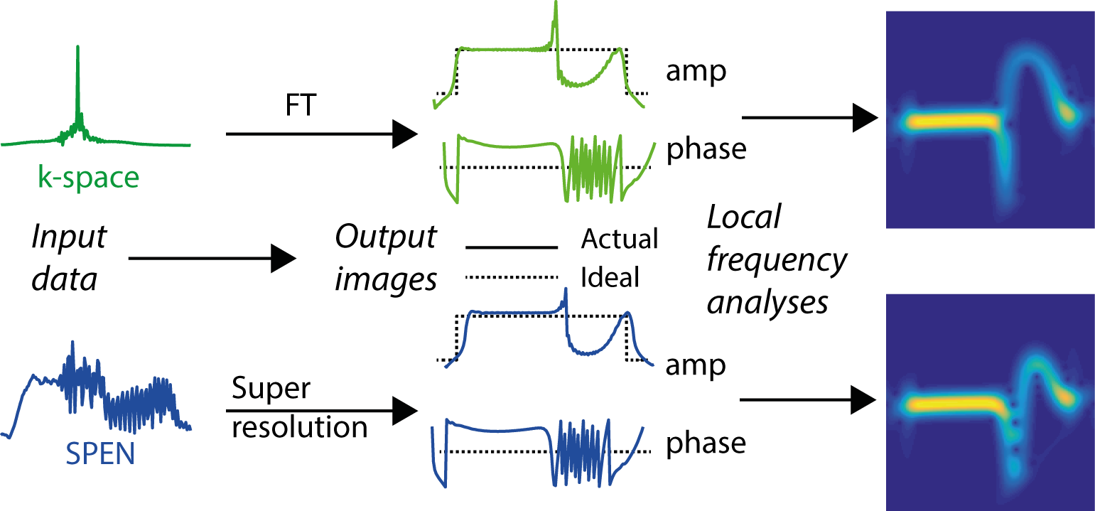
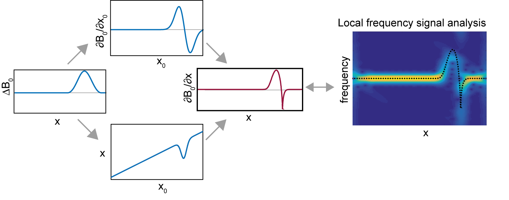
Consider a 1D ΔB0(x) affecting either EPI or SPEN I(x) images. Regardless of the technique there will be a processing protocol that transforms the collected signals into reconstructed images (Fig.1, center). Assume this proceeds in a “B0-agnostic” way, without accounting for ΔB0. Images will then distort away from their ideal amplitude profiles –which since unknown cannot be used for self-referenced corrections – and so will be their phases. As the latter, however, are a priori known for an ideal case, such deviations can be exploited for estimating the intervening field inhomogeneities. To do so we rely on the fact that if B0(x0) is smooth and small enough for avoiding phase-wraps within a voxel, a local frequency analysis of I(x) will retrieve the spectrum that, within the neighborhood of each x, dominates the ΔB0-deviations (Fig. 1, right). The maximum adopted by this frequency spectrum, Δνmax(x), will then be given by the ΔB0 dislocation of ideal x0’s into x’s, and by the frequency variations over a small local region in the neighborhood of these x’s –i.e., the derivatives ∂B0/∂x. Figure 2 illustrates how these two contributions are related to the Δνmax(x) extracted from the function arising after the local frequency analysis of I(x).
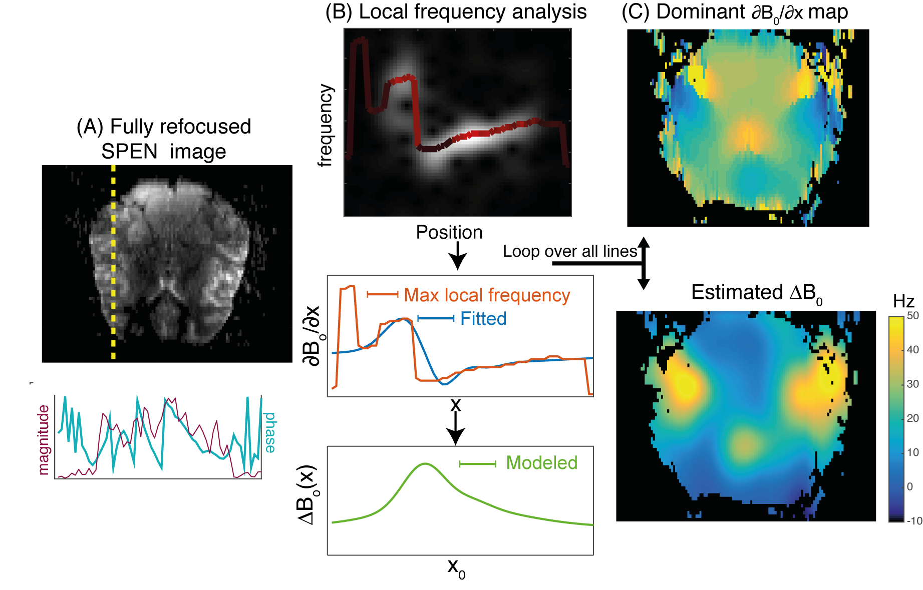
With this as background, Figure 3 illustrates the workflow implemented in this study for extracting ΔB0 from Δνmax(x), focusing for simplicity on SPEN experiments. The 1D analysis in Figures 1 and 2 was done separately on the phase-encoded (x) lines for each readout (y) location. Image lines were subject to a local frequency analysis based on the Gabor transformation6,7 (even if other options are available and are expected to produce similar results). This provides the dominant frequency that for each (dislocated) x-position in the sample, characterizes ∂[B0(x)]/∂x. Rather than integrating this vector and calculating from it the dominant ΔB0(x), we searched for the smooth offsets [γΔB0(x)]calc, that could recreate the experimentally-derived patterns. To this end each [ΔB0(x)]calc was expressed as a sum of three spatial Gaussians, and a cost function Cost(x) = rms{[∂B0/∂x]calc, [∂Bo/∂x]expt} that included a penalty on the amplitude of the Gaussians to encourage simple solutions.
To verify the usefulness of this analysis, healthy human volunteers were scanned in a 3T Siemens TrioTIM MRI after suitable consent. Single-shot fully-refocused SPEN images8 with BW=4.4 kHz were collected, focusing on the lower parts of the temporal lobe and on the prefrontal cortex, as these are brain areas commonly suffering from field inhomogeneities.
RESULTS
Figure 4 summarizes results arising from the present ΔB0 analysis. For each spatial location the analysis clearly reveals a dominant value, which when processed as described above delivers ΔB0 maps typical for this brain region (Fig. 3C). Notice the success of the reconstruction despite targeting fully refocused SPEN data that is free from T2* dephasing8, owing to the fact that the analysis does not focus on the signal at a single point but within a neighborhood of (dislocated) positions.DISCUSSION & CONCLUSION
A new way to evaluate the effects of B0 inhomogeneities commonly encountered in ultrafast imaging was discussed. The scheme can be easily implemented and does not require additional scans or data –even if its success is confined to limited local distortions. The information afforded by this procedure can be used to calculate ΔB0(r), which when fed into image-correction algorithms based on ΔB0(r)–maps can reinstate the image’s faithfulness.Acknowledgements
We are grateful to Dr. Sagit Shushan (Wolfson MC) and Edna Furman-Haran (Weizmann) for assistance. SfC thanks the Feinberg Graduate School (Weizmann) and French Foreign Service for partial postdoctoral fellowships. Support came from the Israel Science Foundation (#2508/17), the EU ERC-2016-PoC grant # 751106, the Minerva foundation (#712277), the Kimmel Institute for Magnetic Resonance and the generosity of the Perlman Family Foundation.References
1. Stehling, M.K., Turner, R., Mansfield, P., 1991. Echo-Planar Imaging: Magnetic Resonance Imaging in a Fraction of Second. Science 254, 43.
2. Tal, A., Frydman, L., 2006. Spatial encoding and the single-scan acquisition of high definition MR images in inhomogeneous fields. Journal of Magnetic Resonance 182, 179–194. doi:10.1016/j.jmr.2006.06.022
3. Jezzard, P., Clare, S., 1999. Sources of distortion in functional MRI data. Human Brain Mapping 8, 80–85.
4. Ben-Eliezer, N., Solomon, E., Harel, E., Nevo, N., & Frydman, L. (2012). Fully refocused multi-shot spatiotemporally encoded MRI: robust imaging in the presence of metallic implants. Magnetic Resonance Materials in Physics, Biology and Medicine, 25(6), 433-442.
5. Jezzard, P., Balaban, R.S., 1995. Correction for geometric distortion in echo planar images from B0 field variations. Magnetic Resonance in Medicine 34, 65–73.
6. Feichtinger, H. G., & Kozek, W. (1998). Quantization of TF lattice-invariant operators on elementary LCA groups. In Gabor analysis and algorithms (pp. 233-266). Birkhäuser Boston.
7. Gröchenig, K. (2013). Foundations of time-frequency analysis. Springer Science & Business Media.
8. Schmidt R, Frydman L. New spatiotemporal approaches for fully refocused, multislice ultrafast 2D MRI. Magn Reson Med 2014;71(2):711-722.
Figures