4210
Improved thermal modelling and prediction of gradient response using sensor placement guided by infrared photography1Information Technology and Electrical Engineering, ETH Zurich, Zurich, Switzerland, 2Skope Magnetic Resonance Technologies AG, Zurich, Switzerland
Synopsis
In MRI, the dynamics of gradient fields can be predicted by assuming that the system is linear and time-invariant. However, time-invariance can be violated by thermal effects. To address this shortcoming, it has been proposed to expand the GIRF model by thermal variation parametrized with the help of temperature sensors. It has remained open how many relevant thermal degrees of freedom the system actually had and where the matching number of sensors should be placed to capture them. In the present work, we address these questions using infrared photography and principal component analysis of gradient heating. Response modelling is additionally enhanced by accelerating GIRF measurements and including cross-terms. The improvements are shown in the prediction of gradient waveforms for image reconstruction and in the effects on the images.
Introduction
In MRI, the dynamics of gradient fields are subject to a range of imperfections, including eddy currents, mutual coupling of gradient coils, and mechanical oscillations. To the degree that these effects are linear and time-invariant they can be described by a matrix of gradient impulse response functions (GIRFs)1,2. However, time-invariance can be violated by thermal effects3. To address this shortcoming, it has been proposed to expand the GIRF model by thermal variation parametrized with the help of temperature sensors4. However, the demonstration of this approach has been limited to few built-in sensors in fixed positions. Thus it has remained open how many relevant thermal degrees of freedom the system actually had and where the matching number of sensors should be placed to capture them. In the present work, we address these questions using infrared photography and principal component analysis (PCA) of gradient heating. Response modelling is additionally enhanced by accelerating GIRF measurements and including cross-terms.Methods
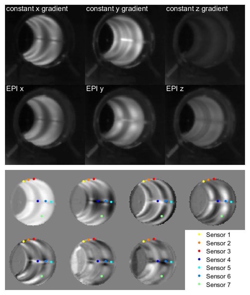
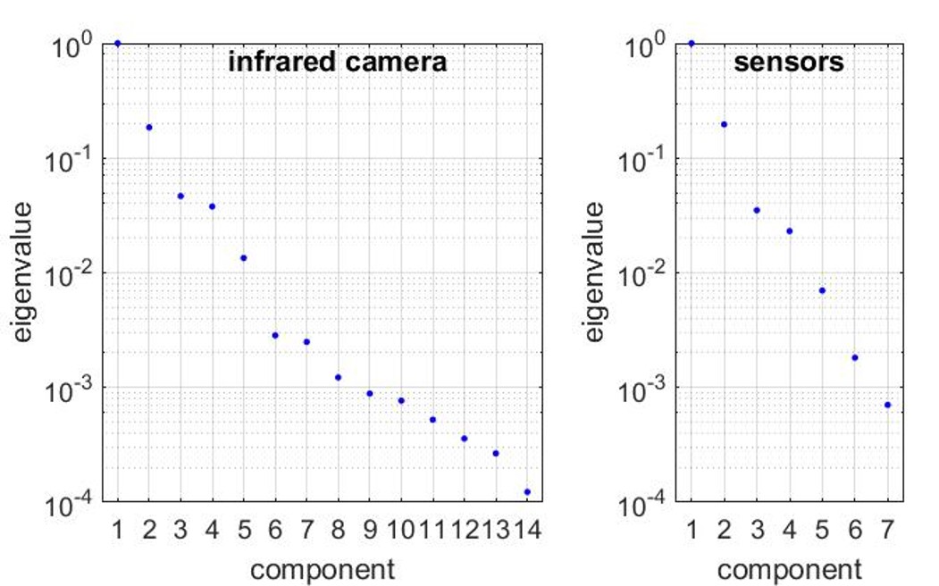
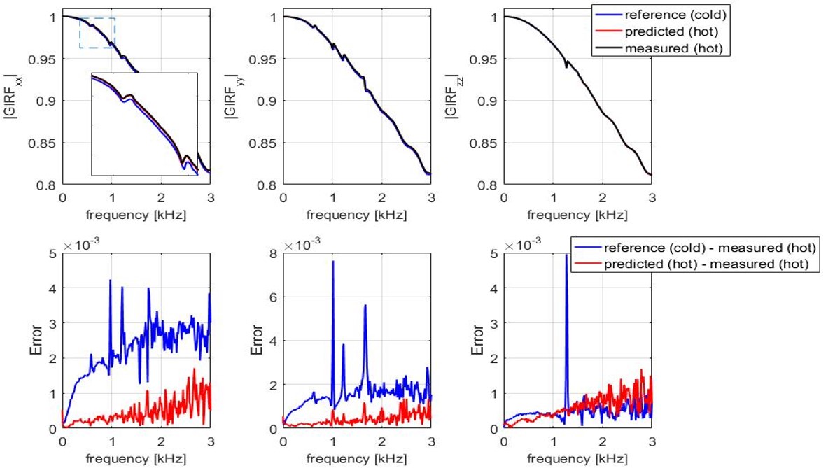
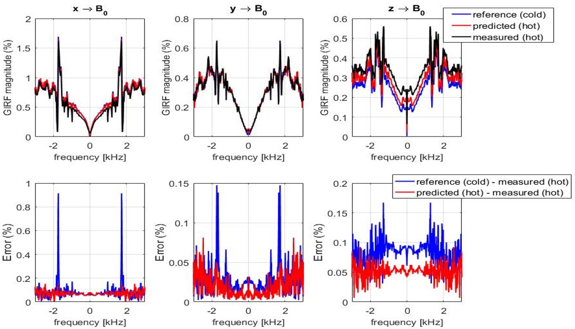
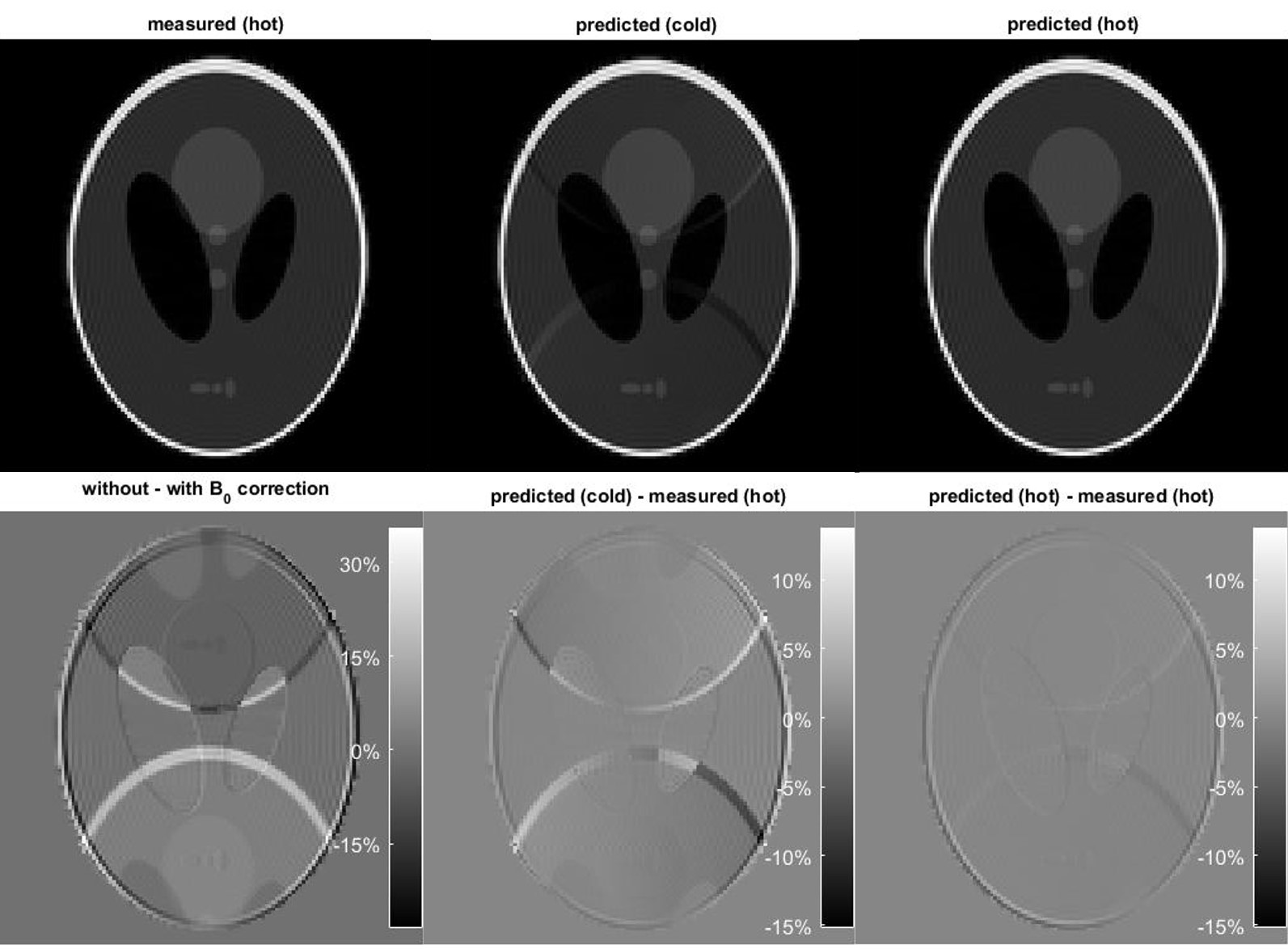
All experiments were performed with a commercial 3T imager (Achieva, Philips Healthcare). The body RF coil was removed and the inner surface of the gradient tube was observed with an infrared camera (Seek Thermal, California, USA). Six different patterns of gradient operation were carried out and the corresponding heating time courses were recorded. Thereafter, the infrared data was subject to principal component analysis. Based on this data, the number of sensors was selected and their positions were set where the respective number of dominant principal components exhibited the greatest variation. This setup was implemented by taping fluoroptic sensors (Neoptix, Canada) to the inside of the gradient tube. It was verified by sensor recordings during an alternate set of test protocols and comparing the eigenvalue spread of their PCA with that of the infrared recordings. Gradient response functions were measured as in Ref. [5], yet using faster frequency sweeps of only 40ms (0-30kHz, maximum field strength: 31mT/m). Field responses were recorded for 70ms with a third-order field camera6 (Skope Magnetic Resonance Technologies) and GIRFs were calculated as described in1. As a basis for thermal modelling, temporally resolved GIRF measurement and concurrent temperature monitoring were performed over 3 hours, using a variety of common scan protocols. The thermal GIRF model was then constructed as in4, using the row vector of 7 temperatures and its time derivative, as parameters. Predictions were carried out for all gradient self-terms and for cross-terms to B0. To assess the scale of gradient response errors at the image level, EPI readouts (resolution=2mm, FOV=256mm, duration=70ms) were simulated based on a k-space trajectory and B0 dynamics obtained by measurement in a hot gradient state. Image reconstruction was then performed using k-space trajectories and B0 dynamics based on cold and hot GIRF prediction as well as the measured field evolution.Results
The different patterns of gradient input resulted in distinct heating patterns on the gradient tube (Fig.1). PCA showed that the thermal variation over time permits expansion into few components (Figs.1,2). Based on the eigenvalue spread, the number of sensors was set to 7, capturing contributions down to almost 1 per mil in terms of variance. PCA of the sensor data yielded only slightly expanded eigenvalue spread (Fig.2), indicating that the sensors capture the first seven thermal degrees of freedom almost optimally. The thermal GIRF model generated with this sensor configuration permitted rather accurate prediction of the self-terms as well as the 0th-order cross-term responses in heated states as shown by examples in Figs.3,4. Alteration of mechanical resonances, in particular, is well predicted. The noise floor increasing with frequency is due to rapid GIRF measurement and present in both the training data and the measurement performed for validation. In the imaging simulations (Fig.5), using the conventional ‘cold’ GIRF model for reconstruction in the hot state yields ghosting artefact, illustrating that thermal changes are of relevant magnitude. The accuracy of the thermal model is illustrated by near-complete removal of ghosting when determining self- and cross-term GIRFs based on actual temperatures.Discussion/Conclusion
The results of this work indicate that relatively few temperature sensors, when well positioned, can capture the thermal degrees of freedom of contemporary gradient tubes to a large degree. Thermal modelling on this basis was found to permit more accurate prediction not only of k-space trajectories but also of B0 cross-term responses. Thermal modelling was facilitated by rapid, time-resolved GIRF measurement, which was explored at a greatly reduced readout time of 70ms. An important advantage of such short readouts is that they permit single-shot GIRF measurement with a single set of long-lived field probes rather than a continuous camera setup with alternate excitation of redundant probe sets7.Acknowledgements
No acknowledgement found.References
[1] S. J. Vannesjo, M. Haeberlin, L. Kasper, M. Pavan, B. J. Wilm, C. Barmet, and K. P. Pruessmann, “Gradient system characterization by impulse response measurements with a dynamic field camera,” Magn. Reson. Med, vol. 69, no. 2, pp. 583–593, 2013.
[2] Addy NO, Wu HH, Nishimura DG. Simple Method for MR Gradient System Characterization. In Proceedings of the 17th Annual Meeting of ISMRM, Honolulu, Hawaii, USA, 2009. p. 3068.
[3] J. Busch, S. J. Vannesjo, C. Barmet, K. P. Pruessmann, and S. Kozerke, “Analysis of temperature dependence of background phase errors in phase-contrast cardiovascular magnetic resonance,” J Cardiovasc Magn Reson, vol. 16, p. 97, 2014.
[4] B. E. Dietrich, J. Nussbaum, B. J. Wilm, J. Reber and K. P. Pruessmann, “Thermal Variation and Temperature- Based Prediction of Gradient Response,” in Proc Int Soc Magn Reson Med Sci Meet Exhib, 2017, p. 0079.
[5] S. J. Vannesjo, B. E. Dietrich, M. Pavan, D. O. Brunner, B. J. Wilm, C. Barmet, and K. P. Pruessmann, “Field camera measurements of gradient and shim impulse responses using frequency sweeps,” Magn. Reson. Med, vol. 72, no. 2, pp. 570–583, 2014.
[6] B. E. Dietrich, D. O. Brunner, B. J. Wilm, C. Barmet, S. Gross, L. Kasper, M. Haeberlin, T. Schmid, S. J. Vannesjo, and K. P. Pruessmann, “A field camera for MR sequence monitoring and system analysis,” Magn. Reson. Med, vol. 75, no. 4, pp. 1831–1840.
[7] B. Dietrich, D. Brunner, B. Wilm, C. Barmet, and K. Pruessmann, “Continuous magnetic field monitoring using rapid re-excitation of NMR probe sets,” IEEE Trans Med Imaging, vol. 35, no. 6, pp. 1452–1462, 2016.
Figures