4209
Using field monitoring to map and correct image distortions due to gradient nonlinearities1Dept. of Radiology, Medical Physics, Medical Center University of Freiburg, Faculty of Medicine, Freiburg, Germany, 2Institute of Biomedical Engineering, National Taiwan University, Taipei, Taiwan
Synopsis
We demonstrate how a field probe array can be used to measure gradient nonlinearities. Brain imaging results show that the distortion was most prominent at image voxels away from the iso-center. Compared to MRI vendor’s solution, our measurements and reconstruction could further reduce the image distortion by 35%.
Introduction
Longitudinal structural brain imaging and quantitative brain morphometry require highly reproducible measurements. However, achieving this requirement with MRI is still a challenge1,2. Subject motion, eddy currents, and magnetic field susceptibility can all introduce image artifacts to deteriorate reproducibility. The gradient non-linearity is one of the prominent sources of image distortion. Images acquired on different days with different subject positioning may be affected by different distortions, which limits non-reproducibility of results. Gradient non-linearity related image distortion is particularly prominent around the edges of the scanner’s imaging volume. They can be corrected using spherical harmonic parameters provided by the vendor. Alternatively, potentially more accurate magnetic field distributions to be used in image reconstruction to correct for distortions can be estimated by image-based methods1-4. However, these methods need specialized phantoms and critically depend on the accuracy of the phantom structure identification. Here, we propose to measure gradient non-linearity by a field probe array with short imaging time. The data can be processed with a simple algorithm to correct for image distortions. We demonstrate that after correction brain structures remain consistent across repeated measurements with varying positioning.Methods
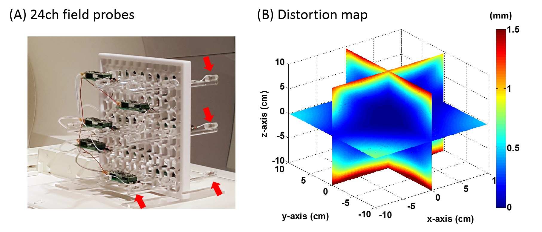
We used a 3D field probe array with 24 probes (Figure 1A), which were arranged in a cubic grid with around 10 cm distance between the probes. The center of the probe array was placed at 3x3x3 different positions, each of which was +3, 0, or -3 cm away from the iso-center in x, y, and z directions. The magnetic field produced by the x, y, and z gradient coils was with the maximal gradient strength of 20 mT/m was mapped and modeled by up to the 5th-order spherical harmonics. Spherical harmonic coefficients were estimated by minimizing the residual between measured and modeled magnetic field at each probe position. A distortion map was then generated based on the estimated spherical harmonic coefficients. Each image was corrected based on the distortion map and interpolated to the target rectangular grid.
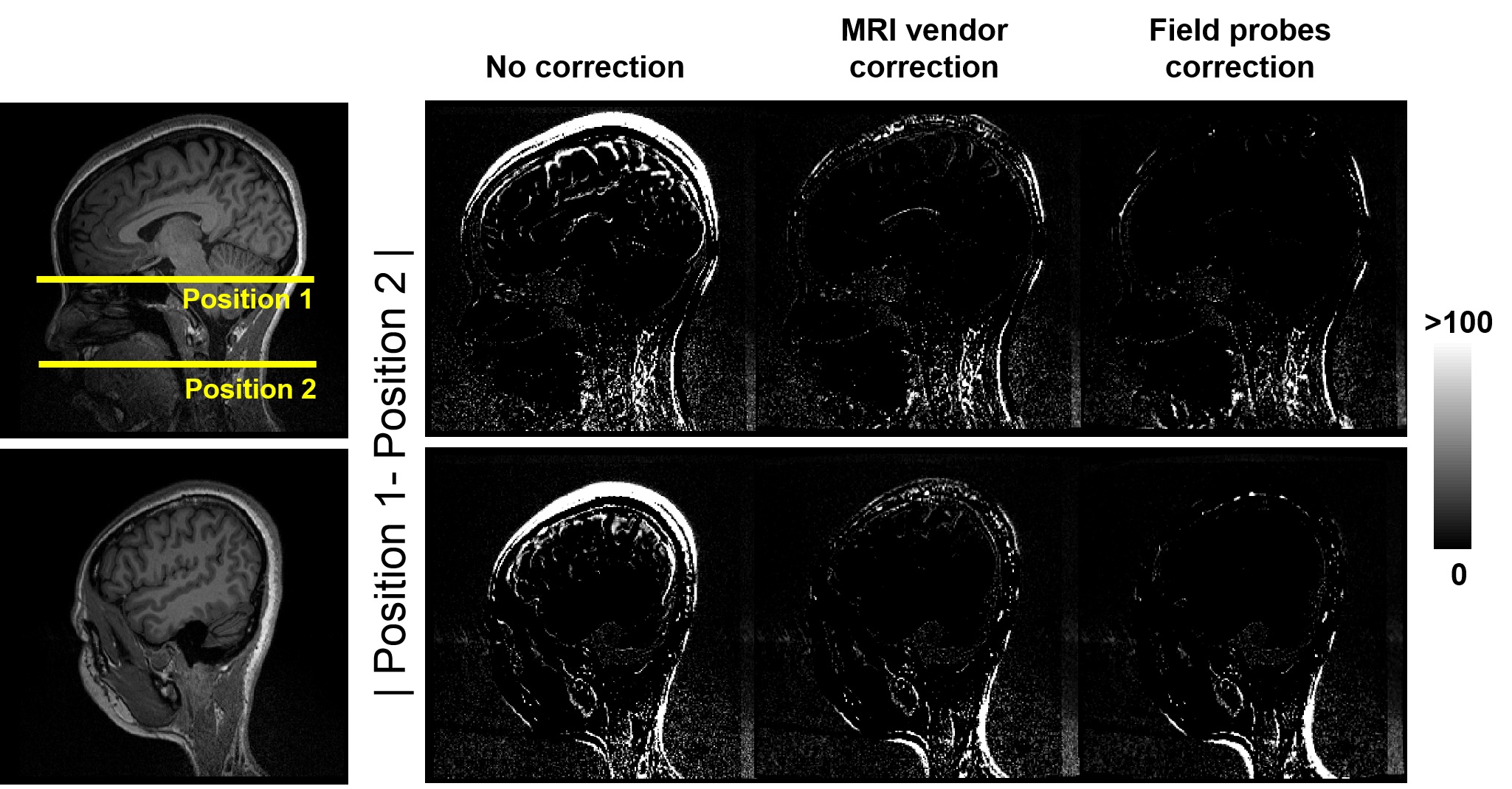
T1-weighted images (MPRAGE: TR=2300ms, TE=2.32ms, resolution=0.9x0.9x0.9mm3) were measured on two different days with the subject in two positions: the magnet iso-center was either near to the eyes (Position 1) or to the mouth (Position 2). The images were reconstructed i) using the 3D distortion correction provided by MRI vendor, and ii) using spherical harmonics estimated by field probes. Thereafter the images were realigned using SPM and analyzed for differences within the brain region. All data were acquired on a 3T MRI system (Prisma, Siemens).
Results
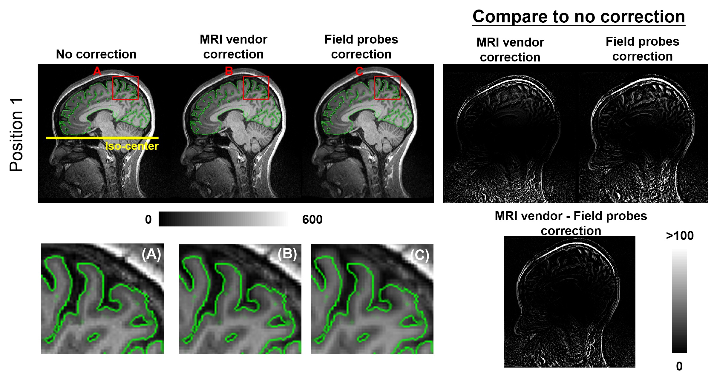
Figure 1B shows a distortion map due to gradient nonlinearly in three orthogonal views. The map illustrates the estimated distance that voxels are shifted because of the gradient nonlinearity. This distance is close to zero near the iso-center and gradually increases towards the periphery of the FOV. As the brain structure is expected to be invariant in two scans, we measured the discrepancies to quantify the effect of image distortion caused by gradient nonlinearity and thereby the performance of distortion correction methods. The l2 norm of the difference image between two scans within the whole brain for no correction, MRI vendor correction, and field probe correction were 34,326, 6,683, and 4,374, respectively. Moreover, there were 13.5%, 5.3% and 1.4% voxels in the brain were not overlapped with each other without correction, with vendor correction, and with probe correction, respectively (Figure 2). At position 1, the structure changes after distortion corrections were shown in Figure 3. Green lines delineate the cortex boundary near the superior central sulcus from the image without correction. This boundary did not align with the cortex boundary after distortion correction which visualizes the effect of applied corrections. The image distortion quantified as the difference before and after correction was more substantial for the scan away from the magnet iso-center. The l2 norm of the difference image between no correction and MRI vendor correction or field probe correction within the whole brain region was 8,596 or 12,389 at Position 1, and 65,420 or 49,787 at Position 2, respectively. Note that the l2-norm of the difference between the two correction methods were 6,567 at Position 1 and 6,886 at Position 2.Discussion
In routine brain scan (at Position 1), the gradient non-linearity can lead to incorrect morphometry quantification and unstable longitudinal structural brain imaging when positions change between scans. However, 80% of geometric distortion caused by gradient non-linearity can be already reduced by MRI vendor correction (l2 norm: 34,326 -> 6,683). Our field probe correction can further reduce this distortion by 35% (l2 norm: 6683 ->4374). There were still noticeable distortion after the gradient nonlinearity correction, we expect this error can be further reduced using higher orders spherical harmonics with denser probe measurements.Acknowledgements
This work was partially supported by Ministry of Science and Technology, Taiwan (103-2628-B-002-002-MY3, 105-2221-E-002-104, 106-2911-I-002-502), and the Academy of Finland (No. 298131).References
1. Caramanos, Z. et al. Gradient distortions in MRI: Characterizing and correcting for their effects on SIENA-generated measures of brain volume change. Neuroimage 49, 1601-1611, doi:10.1016/j.neuroimage.2009.08.008 (2010).
2. Jovicich, J. et al. Reliability in multi-site structural MRI studies: Effects of gradient non-linearity correction on phantom and human data. Neuroimage 30, 436-443, doi:10.1016/j.neuroimage.2005.09.046 (2006).
3. Weavers, P. T. et al. Image-based gradient non-linearity characterization to determine higher-order spherical harmonic coefficients for improved spatial position accuracy in magnetic resonance imaging. Magn Reson Imaging 38, 54-62, doi:10.1016/j.mri.2016.12.020 (2017).
4. Doran, S. J., Charles-Edwards, L., Reinsberg, S. A. & Leach, M. O. A complete distortion correction for MR images: I. Gradient warp correction. Phys Med Biol 50, 1343-1361, doi:10.1088/0031-9155/50/7/001 (2005).
Figures