4207
Extending the Simple Method for Adaptive Gradient-Delay Compensation in Radial MRI1Intistut für Diagnostische und Interventionelle Radiologie, University Medical Center Göttingen, Göttingen, Germany, 2Partner Site Göttingen, German Centre for Cardiovascular Research (DZHK), Göttingen, Germany
Synopsis
Lately, radial k-space trajectories have become very popular especially for fast MRI. However, radial sampling is prone to streaking artifacts caused by gradient delays. Here, we propose two extensions for a simple but powerful method that compensates gradient delays by estimating the corresponding sample shift using cross-correlation of opposed spokes. First, we show that the opposed spokes don't have to be acquired in calibration scans but can be taken directly from the actual measurements. Second, we show that it is also possible to generate synthetic spoke-pairs for gradient delay estimation.
Introduction and Purpose
In the recent years radial k-space sampling has gained increased interest in the MRI community as it provides significant advantages over conventional Cartesian sampling. However, radial MRI sequences require a very precise gradient timing and therefore are prone to eddy-current induced gradient delays which result in k-space miscentering1.
Amongst others2-6, a very simple and popular method for gradient delay correction was introduced by Block and Uecker7. They suggest to calculate the sample shift by performing a cross-correlation of opposed calibration spokes and compensate for it in the gridding procedure. However, this technique requires the acquisition of diametrically opposed spokes prior to the actual measurement. Hence, modifications to an existing radial MRI sequence must be implemented and moreover, the method cannot be applied to measurements with interactive changes to the imaging plane. Here, we reformulate their approach and propose two extensions that don't rely on calibration scans.
Theory
Eddy-currents induce a k-space sample shift which can by modeled using a quadratic form8 (Eq 1) $$ \delta k(\Theta)=\hat{n}^T\left(\begin{array}{cc}S_x&&S_{xy}\\S_{xy}&&S_{y}\end{array}\right)\hat{n},\;\;\hat{n}^T=(\cos{\Theta},\sin{\Theta})$$ with $$$\Theta$$$ the projection angle of the spoke. $$$S_x$$$ and $$$S_y$$$ correspond to the k-space shifts in x and y direction and $$$S_{xy}$$$ accounts for an additional shift induced by the third physical gradient when measuring oblique slices. We propose three related techniques to estimate these parameters:
I) First, we describe a convenient implementation of the method by Block and Uecker7: 1. We sequently acquire calibration spokes $$$P_\Theta$$$ and $$$P_{\Theta -180°}$$$ for various projection angles $$$\Theta$$$ 2. We pick a spoke $$$P_{\Theta}$$$ and its opposed counterpart $$$P_{\Theta-180°}$$$, flip ($$$^f$$$) the latter, Fourier-Transform ($$$\mathcal{F}$$$) both spokes and multiply the $$$\Theta$$$-spoke's transform with the complex conjugate (*) of its flipped counterpart. This yields $$g(r)=\mathcal{F}P_{\Theta}\cdot(\mathcal{F}{P}^{f}_{\Theta-180°})^*,$$ the Fourier-Transform of the cross-correlation function. 3. We calculate the slope of the phase of $$$g(r)$$$ using a scalar product between $$$g(r)$$$ and its duplicate shifted by one pixel $$$g(r+\Delta r)$$$, which magnitude-weights the finite phase-differences. The actual shift is given by $$\delta k(\Theta)=\frac{1}{2}\;\text{arg}(\langle g(r),g(r+\Delta r)\rangle)\;2\pi/(\text{BaseResolution})$$ 4. To obtain $$$S_x$$$, $$$S_y$$$ and $$$S_{xy}$$$, we fit the shifts using the quadratic form (Eq. 1).
In practice it is not always possible or desired to perform calibration scans e.g. if e.g. the imaging plane is interactively changed. We therefore propose two methods that don't rely on calibration scans but use the actual measurement data for shift determination: II) We iterate through all or a subset of acquired spokes and for each spoke we search for the one which is approximately opposed to it. With these (almost) opposed spoke-pairs we can continue with step I.3-4.
III) For highly undersampled radial data there is no guarantee to find sufficiently opposed spokes, thus we generate artificial spoke-pairs by approximating k-space symmetry: $$$P_{\Theta-180°}=P_\Theta^*$$$ and continue with step I.3. In practice, the object appears not necessarily real but has a phase in each channel which we account for in a first order approximation using an extended model (Eq. 2): $$\delta\tilde{k}(\Theta)=\delta{k}(\Theta)+\hat{n}^T\left(\begin{array}{c}D_x\\D_y\end{array}\right)$$ which we use to fit $$$S_x$$$, $$$S_y$$$ and $$$S_{xy}$$$ coil-by-coil and average the results.
Methods
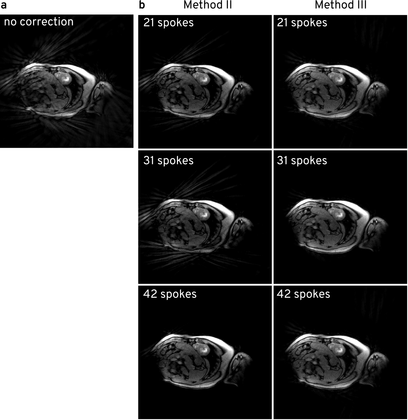
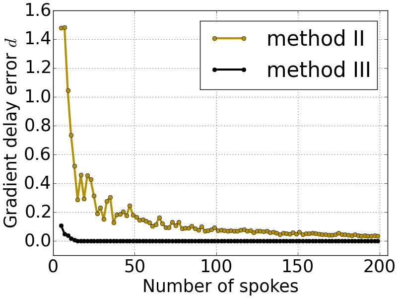
We evaluate the capability of method II and III to eliminate streaking artifacts of a real-time FLASH MRI measurement (FOV = 256x256 mm, base-resolution 256, 21 evenly distributed spokes per frame, 5 interleaved spoke patterns) using 21, 31 and 42 spokes and compare it to a reference without corrections. We furthermore simulate 7-channel radial k-space data with 2 to 200 spokes and mimic the gradient delays $$$S_x=1$$$, $$$S_y=2$$$, $$$S_{xy}=3$$$ by multiplying corresponding phase ramps in the Fourier-domain of the spokes. We use method II and III to recover the generated gradient delays. To measure the error we compare the root-of-squares differences between the actual and estimated shifts.Results and Discussion
Fig. 1 shows one frame of a real-time movie (cardiac short-axis) reconstructed with NLINV9. The depicted preliminary results indicate that streaking artifacts can significantly be reduced using methods II and III. For 42 spokes, method II provides almost perfect gradient delay compensation with III some streakings remain. For very few spokes however, method III provides better results, probably because in II the spoke pairs are not sufficiently opposed. This notion is supported by Fig. 2 which shows that for our simulation the gradient delay estimation error for method III already converges with about 10 spokes whereas the convergence for method II is slower.Conclusion and Outlook
Preliminary results suggest that gradient delay correction can be performed using few spokes of the actual measurement without calibration scans. In the future we will evaluate the robustness of the methods.Acknowledgements
No acknowledgement found.References
[1] Peters, D. C., Derbyshire, J. A. and McVeigh, E. R. (2003), Centering the projection reconstruction trajectory: Reducing gradient delay errors. Magn. Reson. Med., 50: 1–6. doi:10.1002/mrm.10501 [2] Jang, H. and McMillan, A. B. (2017), A rapid and robust gradient measurement technique using dynamic single-point imaging. Magn. Reson. Med., 78: 950–962. doi:10.1002/mrm.26481 [3] Addy, N. O., Wu, H. H. and Nishimura, D. G. (2012), Simple method for MR gradient system characterization and k-space trajectory estimation. Magn. Reson. Med., 68: 120–129. doi:10.1002/mrm.23217 [4] Vannesjo, S. J., Haeberlin, M., Kasper, L., Pavan, M., Wilm, B. J., Barmet, C. and Pruessmann, K. P. (2013), Gradient system characterization by impulse response measurements with a dynamic field camera. Magn Reson Med, 69: 583–593. [5] Jeff H. Duyn, Yihong Yang, Joseph A. Frank, Jan Willem van der Veen, Simple Correction Method fork-Space Trajectory Deviations in MRI, In Journal of Magnetic Resonance, Volume 132, Issue 1, 1998, Pages 150-153, ISSN 1090-7807. [6] Barmet, C., Zanche, N. D. and Pruessmann, K. P. (2008), Spatiotemporal magnetic field monitoring for MR. Magn. Reson. Med., 60: 187–197. doi:10.1002/mrm.21603 [7] Block, K. T. and Uecker, M. (2011), Simple method for adaptive gradient-delay compensation in radial MRI. In: Proceedings of the 19th Annual Meeting of ISMRM, Montreal, Canada, 2816. [8] Moussavi, A., Untenberger, M., Uecker, M. and Frahm, J. (2014), Correction of gradient-induced phase errors in radial MRI. Magn. Reson. Med, 71: 308–312. doi:10.1002/mrm.24643 [9] Uecker, M., Hohage, T., Block, K. T. and Frahm, J. (2008), Image reconstruction by regularized nonlinear inversion—Joint estimation of coil sensitivities and image content. Magn. Reson. Med., 60: 674–682. doi:10.1002/mrm.21691
Figures