4206

Fast eddy current characterization for the development of in-bore devices

David Otto Brunner^1,2, Betram Jakob Wilm^1,2, Simon Gross¹, Benjamin Emmanuel Dietrich¹, Christoph Barmet^1,2, and Klaas Paul Pruessmann¹

¹Institute for Biomedical Engineering, ETH and University of Zurich, Zurich, Switzerland, ²Skope Magnetic Resonance Technologies Inc., Zurich, Switzerland

Synopsis

Devices operating in the magnet bore, such as coil arrays, receivers or shim inserts become ever more sophisticated as well as the employed image acquisition schemes. However, quantitative testing for their influence on the gradient switching performance is often difficult and time consuming. In this work we present a methodology for measuring, evaluating and predicting eddy current effects fast and quantitatively, employing a dynamic magnetic field camera and a framework of linear time invariant system characterization. For demonstration, standard components and several frequently applied RF coils are assessed.

Introduction

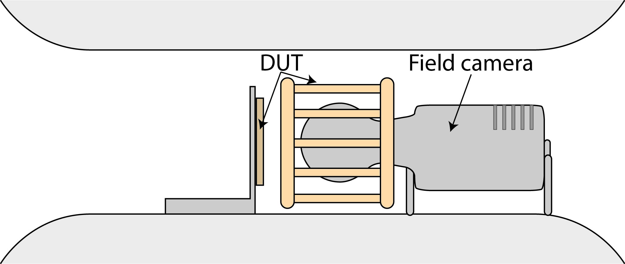
Ever more sophisticated devices are being used in MR imaging, such as high-density receive coils, $$$B_0$$$-shim inserts [1] or combined RF and shimming arrays [2]. All devices require careful testing for electromagnetic compatibility with the MRI system and its protocols. Typical procedures employ the imaging capabilities of the scanner to detect potentially occurring problems such as $$$B_1^+$$$ degradation, static $$$B_0$$$ distortions or added noise. However, it is difficult to assess if a device impacts the accuracy of the gradients by carrying eddy currents. Although the typically performed evaluation of artefacts of demanding read-outs (e.g. EPI) allows determining overall adequacy for the particular sequence, it is difficult to ascribe each artefact to unwanted interactions of the device and the gradient system and to localize and quantify the cause of the problem. This is because gradient distortions interfere with the encoding and corrections required for the acquisition of the validation data itself resulting in a complicated entanglement of various effects. Additionally, an evaluation [3] is most valuable during development but at the same time particularly difficult to perform if not all resources are fully operational. The assessment of the suitability of devices and components remains therefore largely based on the experience of developers. As a solution, we present a framework to measure and to quantify the effect of a device on the spatio-temporal gradient accuracy working independently from the scanner by employing a dynamic field camera (Fig. 1) and signal models based on linear time-invariant systems (LTI) theory. Based on this analysis the source of the distortions can be localized and the impact on image acquisitions can be quantitatively predicted.

Methods

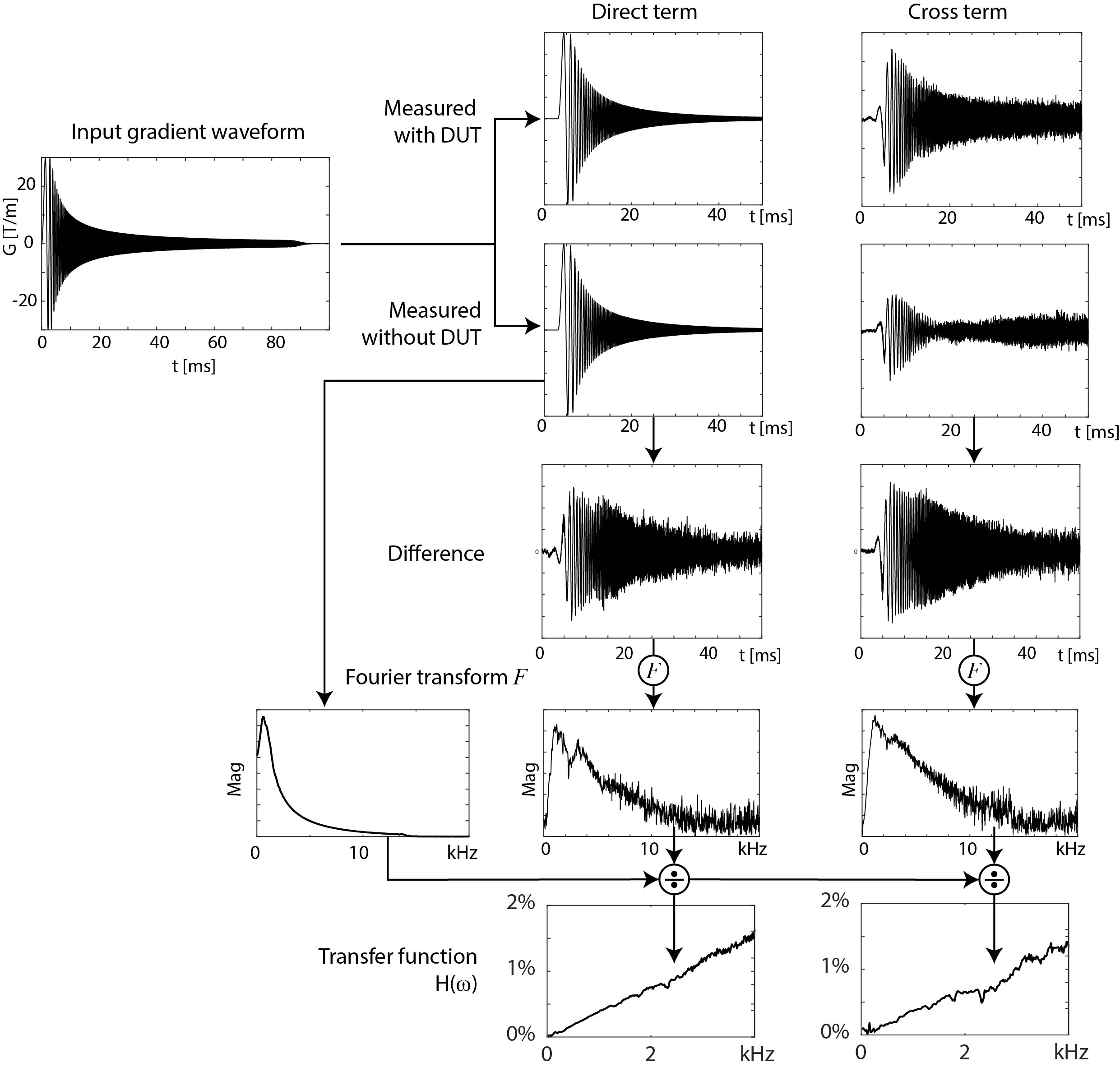
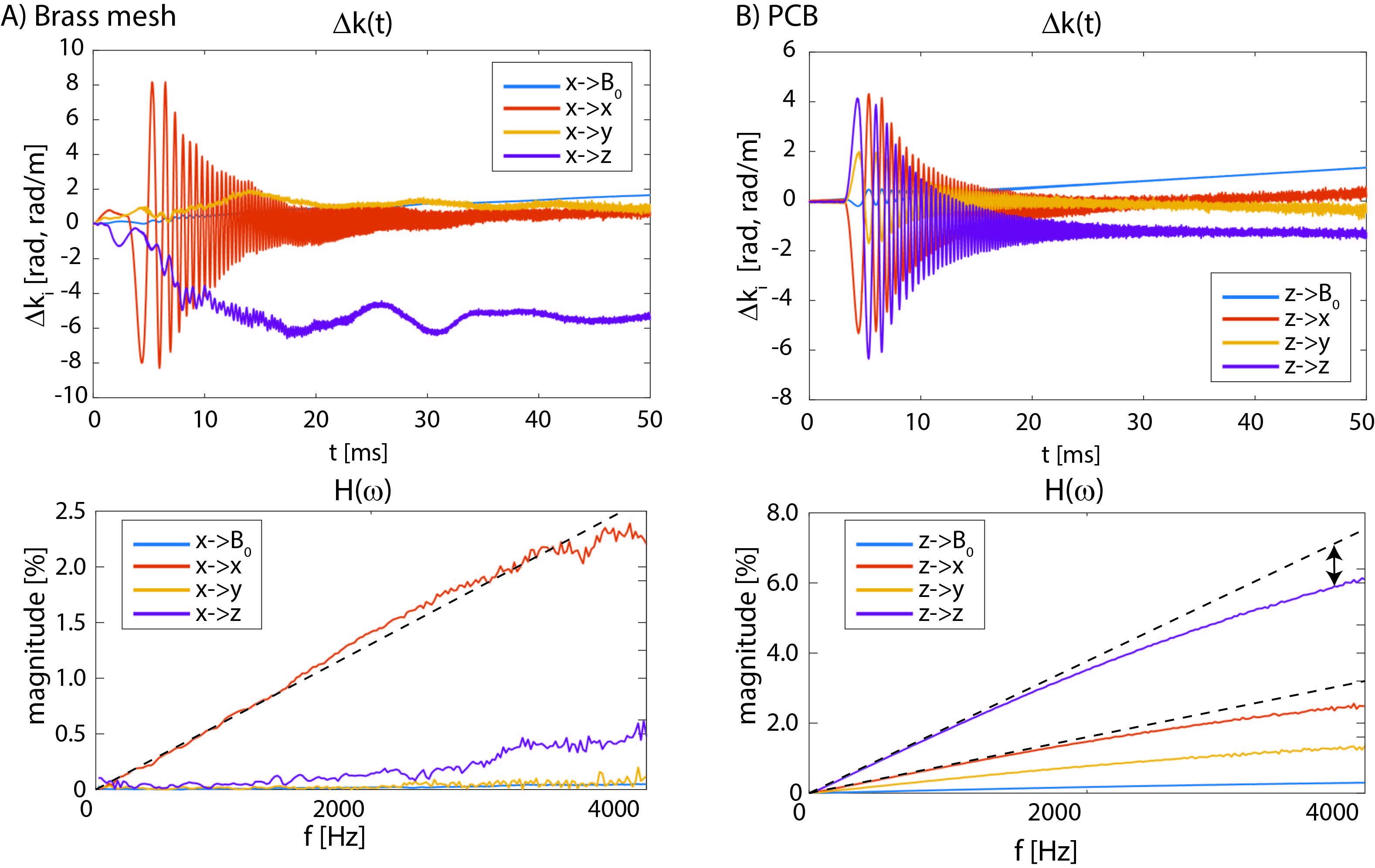
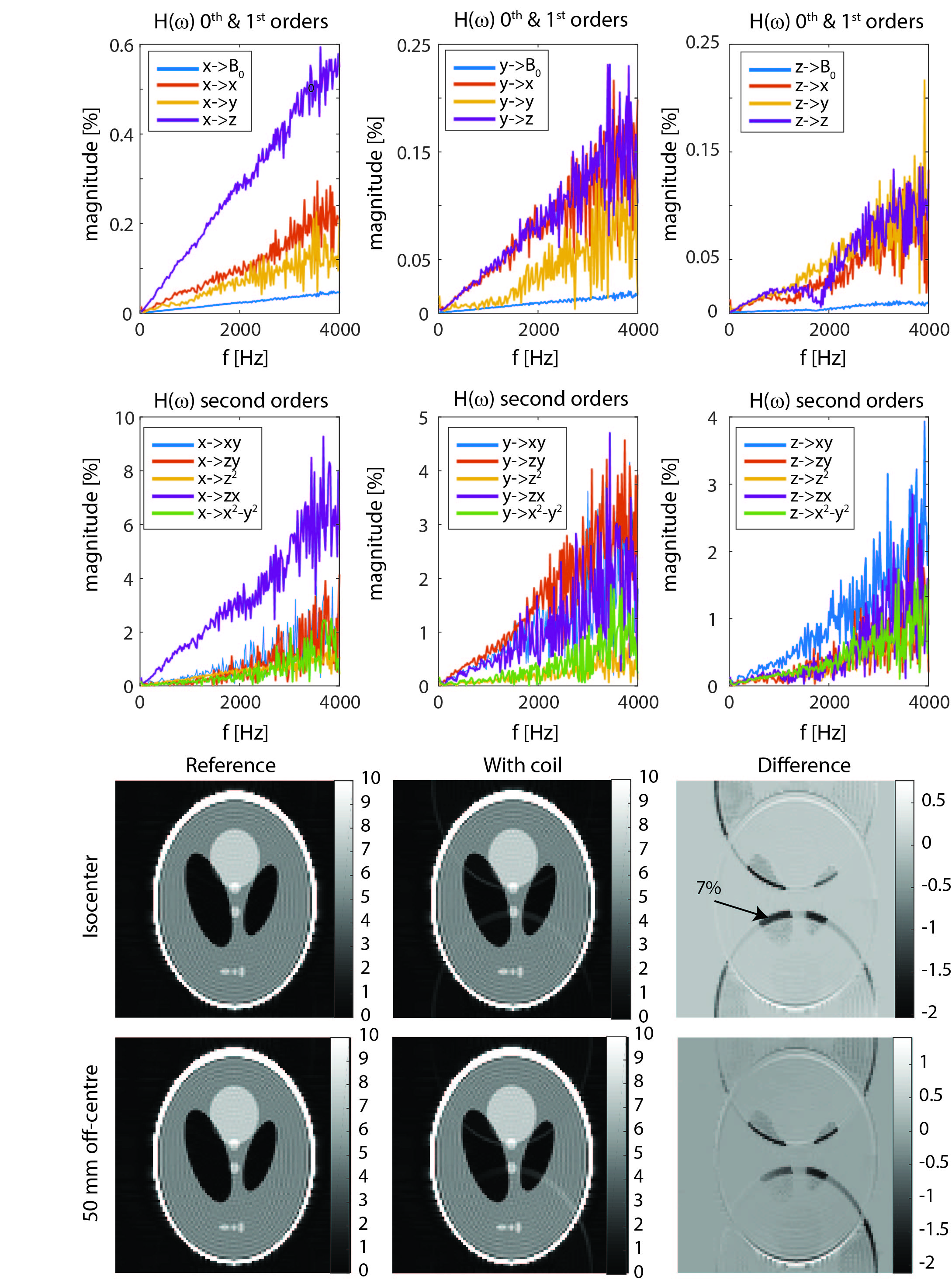
The fields ($$$B_{DUT}(\omega)= F(b_{DUT}(t))$$$) produced by eddy currents on the DUT’s (Device Under Test) conductors, being small compared to the gradient fields, are treated as a perturbation of the system without DUT ($$$B_{ref}$$$). Such an LTI is characterized by its impulse response ($$$h_{DUT}(t)$$$) or its Fourier transform, the transfer function $$$H_{DUT} (\omega)=F(h_{DUT} (t))$$$ [4]: $$b_{DUT}(\vec r, t)=b_{ref}(\vec r,t) \otimes h_{DUT} (\vec r, t)=F(B_{ref}(\vec r, \omega) \cdot H_{DUT} (\vec r, \omega)).$$ Spherical harmonic functions ($$$Y_{l,m}(\vec r)$$$) are employed for capturing the spatial distribution of the field: $$ b_{DUT} (\vec r, t)=\sum_{l’,m’}b_{DUT} (t)\cdot Y_{l’,m’}(\vec r)=\sum_{l’,m’} Y_{l’,m’}(\vec r) \sum_{l,m} ( h_{DUT}^{l,m->l’,m’}(t) \otimes b_{ref}^{l,m}(t)).$$ Acquiring the field evolution with DUT ($$$b_{tot}=b_{DUT}+b_{ref}$$$) and without while driving frequency sweeps subsequently on all axes yields the transfer functions: $$ H_{DUT}^{l,m->l’,m’}(\omega)=F(h_{DUT}^{l,m->l’,m’}(t))=\frac{B_{tot}^{l’,m’}(\omega)- B_{ref}^{l’,m’}(\omega)}{ B_{ref}^{l,m}(\omega)}.$$ A field camera [6] (DFC-16, Skope AG, Zurich, Switzerland) is employed in a 3T scanner (Achieva, Philips Healthcare, Best, Netherlands). As DUT components such as a brass mesh, a PCB and two commercial coils, a TR head-birdcage and an 8-channel receive-only head-array, have been employed. For illustration, image acquisitions have been simulated using the measured reference impulse responses and reconstructed using that of the scanner with the coil.

Results

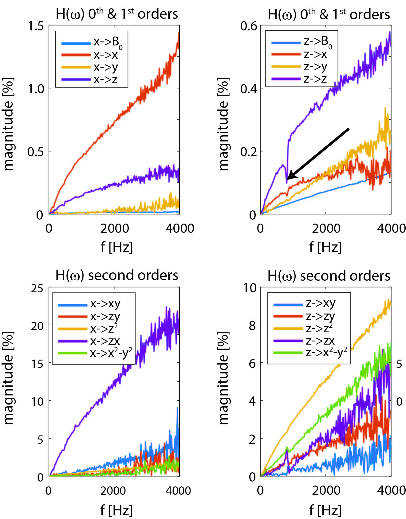
See Figures 3-5.

Conclusion

The proposed measurement of the transfer function of devices gives detailed insight into the spatio-temporal field distortions induced during scanning. Forward calculation of the field evolution employing the response of the scanner and the device allows evaluating the imaging performance time and cost effectively in-silico for all sequences and in principle for various scanners. Similarly, the measurements of the properties of isolated components can predict the behaviour of the entire assembly. These abilities grow ever-more useful, as in-bore deployed setups become more sophisticated and the gradient systems more performant while the requirements on image quality and quantitation are steadily growing. In addition, the captured spatial distribution of the distorting fields allows localizing its source. The frequency response relates to the lifetime of the eddy currents and the mechanical response of the device being determined by the geometry and the involved materials’ properties. Such information is key for determining the source of the problem and improving the design, but difficult to predict otherwise since all, material parameters, their macroscopic assembly and the interaction with the various scanner induced fields have to be accounted for in detail. Doing so at an early design stage is valuable in minimizing development time. The distortions induced by standard coils varied strongly and can generate visible effects in advanced protocols. While EPI phase correction [7] and other delay compensations [8] can largely correct for direct terms, cross terms require more advanced eddy current compensation schemes even involving dynamic shimming for higher orders. Hence, it is imperative to minimize perturbations by hardware design in the first place, especially for use in high-performing gradient systems.

Acknowledgements

No acknowledgement found.

References

1. C. Juchem, et al., Dynamic Multi-Coil Technique (DYNAMITE) Shimming of the Rat Brain at 11.7 Tesla. NMR Biomed, 2014. 27(8).

2. J.P. Stockmann, et al., A 32-channel combined RF and B0 shim array for 3T brain imaging. Magn Reson Med, 2015

3. M. Alecci, et al., Characterization and reduction of gradient-induced eddy currents in the RF shield of a TEM resonator. Magn Reson Med, 2002. 48(2).

4. S.J. Vannesjo, et al., Gradient and shim pre-emphasis by inversion of a linear time-invariant system model. Magn Reson Med, 2016

5. J. Busch, et al., Analysis of temperature dependence of background phase errors in phase-contrast cardiovascular magnetic resonance. Journal of Cardiovascular Magnetic Resonance, 2014. 16(1).

6. B.E. Dietrich, et al. An Autonomous System for Continuous Field Monitoring with Interleaved Probe Sets. in Proc Int Soc Magn Reson Med. 2011 p. 1842.

7. P. Jezzard, et al., Characterization of and correction for eddy current artifacts in echo planar diffusion imaging. Magn Reson Med, 1998. 39(5).

8. N.-k. Chen, et al., Removal of EPI Nyquist ghost artifacts with two-dimensional phase correction. Magn Reson Med, 2004. 51(6).

Figures

Figure 1: Measurement setup: The Dynamic Field Camera (DFC) is positioned in the imaging region for the acquisition of the reference field evolution. Then the device under test (DUT) is placed in the position of planned use for the second acquisition. The DFC acquires the magnetic field evolution up to third spatial order while the scanner plays out a test frequency sweep on each gradient axis or shimming coil subsequently. Each acquisition lasted 100 ms, 10 repetitions were acquired.

Figure 2: Data evaluation path: The scanner is programmed to play out a frequency sweep on each gradient axis. The field evolution is acquired up to third order in space (described by 16 phase coefficients k0 – k15), once with and once without DUT. The difference in the corresponding field evolution is deconvolved with the measured field evolution of the main driving term by division of their respective windowed Fourier transforms. These transfer functions are calculated for the driving axes onto themselves (direct terms) and for field evolutions coupling to different spatial orders (cross terms).

Figure 3: Example data sets (0th and 1st order) acquired using a brass mesh (A) and an unslotted copper circuit board (B) as DUTs. Upper row: DUT induced deviations of monitored k-space trajectory during the sweep. Below: Magnitude of the transfer functions. As expected for eddy current induction, the response is 0 at DC and increases with frequency. The PCB shows a stronger response which is not linearly increasing with frequency as indicated by the dotted lines. The latter effect can be attributed to a longer eddy current life-time on the PCB compared to the mesh.

Figure 4: Selected transfer functions of the T/R head coil. Top row: Response of the x (AP) and the z (FH) gradient to the fields of zeroth and first spatial order. Bottom: Cross terms to the second order fields. Substantial eddy currents can be seen primarily in the same direction as the exciting gradient probably caused by the end-cap shielding of the coil. A sharp dip in the z->z response (arrow) indicates a mechanical resonance of the coil housing.

Figure 5: Transfer functions of eddy currents induced by the eight-channel receive array. In comparison to the T/R coil, the linear response terms are an order of magnitude lower and linearly increasing with frequency suggesting smaller and thinner conductive areas. The perturbing fields point mainly in z with an asymmetric response on x and y localizing the conductor at the head-end and its bottom. Their effect on a simulated single-shot EPI (230mm FOV, 2 mm resolution, 60ms readout) acquisition is shown by the image series at the bottom where a ghost of up to 7% would occur without phase correction.

Proc. Intl. Soc. Mag. Reson. Med. 26 (2018)

4206