4202
Motion Encoding Gradient Nonlinearity Correction for Magnetic Resonance Elastography1Mayo Clinic, Rochester, MN, United States, 2General Electric Global Research Center, Niskayuna, NY, United States
Synopsis
Due to engineering limitations, the spatial encoding gradient fields produced by an MRI scanner are never perfectly linear. Gradient non-ideality is typically associated with image geometric distortion, but it also imparts spatially varying bias in the signal generated during gradient-based motion encoding. In this work, we theoretically investigate how motion encoding gradient nonlinearity affects MR elastography and develop a corrective strategy applicable to any MRE protocol.
Introduction
Due to engineering limitations, the spatial encoding gradient fields produced by an MRI scanner are never perfectly linear. Gradient nonlinearity is typically associated with image geometric distortion; however, it also spatially biases motion-encoding-gradient (MEG) generated signals. While this effect has been studied in diffusion1 and phase-contrast flow2, how MEG nonlinearity impacts MR elastography3 (MRE) has not been reported, to our knowledge. In this work, we theoretically investigate this scenario and develop a corrective strategy for MRE phase data. The non-triviality of this effect is demonstrated on a Compact 3T MRI system employing high-performance gradients that are advantageous for elastography5,6.Theory
In a standard scan, the spatial encoding field at position $$$\vec{r}=x\vec{i}+y\vec{j}+z\vec{k}$$$ is conventionally modeled as
$$B(\vec{r},t) = S_{X}(\vec{r})G_{X}(t) + S_{Y}(\vec{r})G_{Y}(t) + S_{Z}(\vec{r})G_{Z}(t) = \mathbf{G}(t)^{T}\mathbf{S}(\vec{r})~[EQ1]$$
where $$$G_{D}(t)$$$ is the (normalized) gradient waveform for direction $$$D$$$, and $$$S_{D}$$$ is the coil spatial response function, modeled as a low-order spherical harmonic expansion7. $$$S_{D}$$$ ideally varies linearly and only within its nominal dimension (e.g., $$$S_{X}(\vec{r})=x$$$); however, in practice, fields vary nonlinearly and in all directions.
Presuming [EQ1], the $$$n^{th}$$$ k-space measurement is modeled as
$$g[n]=\int_{\Omega}m_{0}(\vec{r})e^{-j\phi(\vec{r})}e^{-j\mathbf{k}[n]^{T}\mathbf{S}(\vec{r})}d\vec{r}~[EQ2]$$
where $$$m_{0}$$$ is spin density, $$$\mathbf{k}[n]$$$ is the k-space vector (i.e., time-integral of $$$\mathbf{G}(t)$$$ during readout ($$$t\geq{\Delta}$$$)), and $$$\phi(\vec{r})$$$ is motion encoded phase, the target quantity in MRE. The phase-modulated image $$$\hat{m}_{0}(\vec{r})=m_{0}(\vec{r})e^{-j\phi(\vec{r})}$$$ can be estimated by interpolating8 the inverse Fourier transform of $$$g$$$ or model-based reconstruction9, from which $$$\phi(\vec{r})$$$ can be extracted.
In MRE, spins move harmonically as $$$\vec{\mu}(\vec{r},t)=\vec{\mu}(\vec{r},0)+\mathrm{Re}\left\{\vec{\eta}_{0}(\vec{r})\exp\left(j\left(\zeta(\vec{r})-\omega{t}+\alpha\right)\right)\right\}$$$, where $$$\vec{\mu}(\vec{r},0)$$$, $$$\vec{\eta}_{0}(\vec{r})$$$, $$$\zeta(\vec{r})$$$, $$$\omega$$$, and $$$\alpha$$$ are peak displacement, instantaneous wave frequency, mechanical driving frequency, and phase delay, respectively. For moving spins, $$$S_{D}(\cdot)$$$ can be approximated (about $$$\vec{r}_{0}$$$) as $$$\mathbf{S}(\vec{\mu}(\vec{r},t))\approx\mathbf{S}(\vec{r}_{0})+\mathcal{J}_\mathbf{S}(\vec{r}_{0})\left(\vec{\mu}(\vec{r},t)-\vec{r}_{0}\right)$$$, where $$$\mathcal{J}_\mathbf{S}(\cdot)$$$ is the Jacobian of the field vector. After simplification, it follows that
$$\phi(\vec{r})\approx-\gamma\mathbf{A}^{T}\left(\mathbf{I}_{2\times{2}}\otimes\mathcal{J}_\mathbf{S}(\vec{r}_{0})\right)\left[\begin{array}{c}\vec{\eta}_{0}(\vec{r})\cos\left(\zeta(\vec{r})\right)\\\vec{\eta}_{0}(\vec{r})\sin\left(\zeta(\vec{r})\right)\end{array}\right]~[EQ3],$$
where $$$\mathcal{F}_\mathbf{G}(\cdot)$$$ is the MEG Fourier transform, $$$\otimes$$$ is Kronecker's product, and
$$\mathbf{A}_{p}=\left[\begin{array}{cc}+\mathrm{Re}\left\{\exp\left(j\alpha\right)\mathcal{F}_\mathbf{G}(\omega)\right\}\\-\mathrm{Im}\left\{\exp\left(j\alpha\right)\mathcal{F}_\mathbf{G}(\omega)\right\}\end{array}\right]~[EQ4].$$
Considering an MRE exam with $$$S$$$ scans (i.e., different MEG directions/offsets), the gradient nonlinearity-corrected first harmonic is estimated via pseudo-inversion ($$$\dagger$$$) as
$$\left[\begin{array}{c}\vec{\eta}_{0}(\vec{r})\cos\left(\zeta(\vec{r})\right)\\\vec{\eta}_{0}(\vec{r})\sin\left(\zeta(\vec{r})\right)\end{array}\right]\approx -\frac{1}{\gamma}\left(\left[\begin{array}{c}\mathbf{A}_{0}^{T} \\\mathbf{A}_{1}^{T} \\\vdots\\\mathbf{A}_{S-1}^{T} \\\end{array}\right]\left(\mathbf{I}_{2\times{2}}\otimes\mathcal{J}_\mathbf{S}(\vec{r}_{0})\right)\right)^{\dagger}\left[\begin{array}{c}\phi_{0}(\vec{r}) \\\phi_{1}(\vec{r}) \\\vdots \\\phi_{S-1}(\vec{r}) \\\end{array}\right]~[EQ5].$$
For MRE, $$$\vec{r}_{0} = \vec{r}$$$ is recommended. [EQ5] applies to any MRE sequence3,10,11,12. However, when MEGs are applied mono-directionally3 for $$$C$$$ cycles with (pseudo-)sinusoidal gradients at amplitude $$$\|\mathbf{G}_{0}\|_{2}$$$, [EQ5] simplifies to
$$\vec{\delta}(\vec{r},n) \approx -\frac{\omega}{\gamma\pi C \left\|\mathbf{G}_{0}\right\|_{2}}\mathcal{J}_\mathbf{S}(\vec{r}_{0})^{\dagger}\left[\begin{array}{c}\phi_{0}(\vec{r}) \\\phi_{1}(\vec{r}) \\\vdots \\\phi_{S-1}(\vec{r}) \\\end{array}\right]~[EQ6],$$
where $$$\vec{\delta}(\vec{r},n)=\vec{\eta}_{0}(\vec{r})\cos\left(\zeta(\vec{r})-\frac{2\pi n}{N}\right)$$$ is the displacement vector at offset $$$n\in[0,N)$$$. Hence, in most cases, MRE phase data (pre- or -post subtraction) can be corrected prior to first harmonic estimation.
Methods
To understand the potential impact gradient nonlinearity has on MRE accuracy, a healthy volunteer was scanned under an IRB-approved protocol on a compact 3T system4,5 (diameter-of-spherical-volume (DSV)=26cm) with real-time concomitant field compensation13,14. A spin-echo echo-planar-imaging (EPI) sequence was modified to include one 18.2ms trapezoidal MEG pair surrounding the RF refocusing pulse with the following parameters: $$$\omega/{2\pi}$$$=60Hz vibration; TR/TE=3600/62ms; FOV=24cm; matrix=72$$$\times$$$72; 48 contiguous 3-mm-thick axial slices; MEG directions=$$$\{±X,±Y,±Z\}$$$; $$$N=8$$$ phase-offsets. Following per-axis phase subtraction, gradient nonlinearity correction ([EQ6]) was performed using vendor-provided distortion coefficients, by modifying previously-described software15,16 for diffusion correction. After correction, MRE post-processing17 comprised: 1) calculating the curl of the displacement images; 2) data smoothing; and 3) stiffness estimation via spatially-adaptive direct inversion.Results
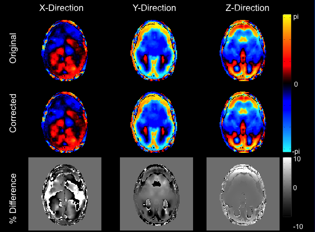
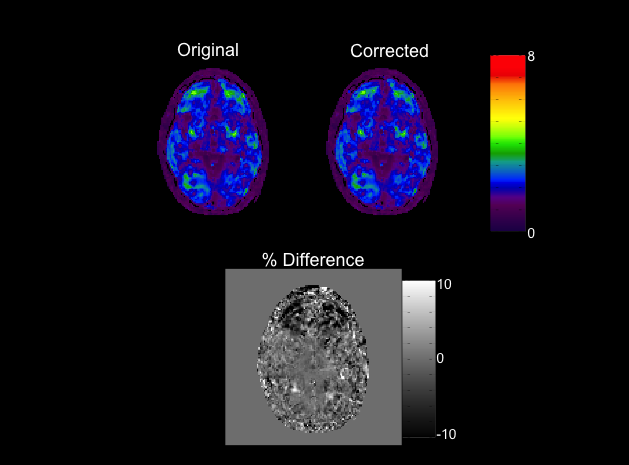
Figure 1 shows raw and gradient nonlinearity-corrected MRE displacement images for each MEG direction at one offset. Although the displacement images are visually similar, per-axis differencing reveals up to 15% changes in values. Difference images were not unwrapped. The increasing impact at distance from isocenter is most evident along the anterior-posterior (AP) direction of the z-component difference image. Figure 2 shows the inversion results for the post-curled displacement image sets. Similar to the images in Figure 1, the effect of gradient nonlinearity on the stiffness results is best visualized within the difference image, where up to 15% decreases in stiffness are observed in the frontal lobe. As a phased-array coil was used in this experiment, the subject's head was slightly shifted anteriorly -- hence, the area of substantial difference coincides with the anatomy experiencing the strongest gradient nonlinearity.Discussion
In this work, we theoretically characterized the effect of MEG nonlinearity in MRE, and developed a universally-applicable correction strategy. On a compact scanner, gradient nonlinearity was observed to cause stiffness changes on the same order as previously associated with disease18. Although this effect is most pronounced when the imaging field-of-view (FOV) approaches the DSV -- e.g., brain imaging on the compact system, or large FOV imaging on whole-body systems -- it nonetheless motivates the need to systematically characterize gradient nonlinearity effects in MRE. Separately, the developed theory can potentially utilized as part of a model-based reconstruction framework, such as previously described for MRE19.Acknowledgements
This work was partially supported by AHA 16POST29900011, and NIH R01-HL115144, R01-EB001981, BRP-R01-EB010065, and U01-EB024450.References
1. Bammer, R., et al. "Analysis and generalized correction of the effect of spatial gradient field distortions in diffusion-weighted imaging." Magnetic resonance in medicine 50.3 (2003): 560-569.
2. Markl, M., et al. "Generalized reconstruction of phase contrast MRI: analysis and correction of the effect of gradient field distortions." Magnetic resonance in medicine 50.4 (2003): 791-801.
3. Muthupillai, R., et al. "Magnetic resonance elastography by direct visualization of propagating acoustic strain waves." Science(1995): 1854-1857.
4. Weavers, Paul T., et al. "Compact three-tesla magnetic resonance imager with high-performance gradients passes ACR image quality and acoustic noise tests." Medical physics 43.3 (2016): 1259-1264
5. Arani, Arvin et al. "High Resolution 3D FGRE is Feasible for Brain MR Elastography with High Performance Compact 3T Scanner", Proceedings of the ISMRM 2017, p.1367.
6. Tan ET, Lee S-K, Weavers PT, Graziani D, Piel JE, Shu Y, Huston J, Bernstein MA, Foo TKF. High slew-rate head-only gradient for improving distortion in echo planar imaging: Preliminary experience. J Magn Reson Imaging 2016;44:653–664.
7. Romeo, Françoise, and D. I. Hoult. "Magnet field profiling: analysis and correcting coil design." Magnetic Resonance in Medicine 1.1 (1984): 44-65.
8. Glover, Gary H., and Norbert J. Pelc. "Method for correcting image distortion due to gradient nonuniformity." U.S. Patent No. 4,591,789. 27 May 1986.
9. Tao, Shengzhen, et al. "Integrated image reconstruction and gradient nonlinearity correction." Magnetic resonance in medicine 74.4 (2015): 1019-1031.
10. Oliphant, Travis E., et al. ``Complex-valued stiffness reconstruction for magnetic resonance elastography by algebraic inversion of the differential equation.'' Magnetic resonance in Medicine 45.2 (2001): 299-310
11. Klatt, Dieter, et al. ``Sample interval modulation for the simultaneous acquisition of displacement vector data in magnetic resonance elastography: theory and application.'' Physics in medicine and biology 58.24 (2013): 8663
12. Grimm, Roger C. et al. ``Gradient Moment Nulling in MR Elastography of the Liver. '' Proceedings of the ISMRM 2007, p.961.
13. Tao, Shengzhen et al., "Gradient Pre-Emphasis Correction for First-Order Concomitant Fields of an Asymmetric Head-Only MRI Gradient System", Magnetic Resonance in Medicine 77(6):2250-2262, 2017.
14. Weavers, Paul T. et al. "B0 concomitant field compensation for MRI systems employing asymmetric transverse gradient coils", Magnetic Resonance in Medicine 38(5):54-62, 2017.
15. Tan, Ek T., et al. "Improved correction for gradient nonlinearity effects in diffusion-weighted imaging." Journal of Magnetic Resonance Imaging 38.2 (2013): 448-453.
16. Tao, Ashley T. et al. "Improving Apparent Diffusion Coefficient Accuracy on a Compact 3T MRI Scanner using Gradient Non-linearity Correction", Proceedings of the ISMRM 2017, p.1396.
17. Murphy Matthew C. et al. "Measuring the characteristic topography of brain stiffness with magnetic resonance elastography". Proceedings of the ISMRM 2013, p.2422.
18. Hiscox, Lucy V., et al. "Magnetic resonance elastography (MRE) of the human brain: technique, findings and clinical applications." Physics in medicine and biology 61.24 (2016): R401.
19. Trzasko, Joshua D. et al. "A Graph Cut Approach to Regularized Harmonic Estimation for Steady-State MR Elastography." Proceedings of the ISMRM 2014, p.4268.
Figures