4170
3D specific absorption rate estimation from focused ultrasound sonications using the Green’s function heat kernel1Radiology and Imaging Sciences, University of Utah, Salt Lake City, UT, United States
Synopsis
In-vivo determination of tissue thermal and acoustic properties, such as the specific absorption rate (SAR) for focus ultrasound, are important for accurate thermal modeling in treatment planning, monitoring, and control using, e.g., Pennes bioheat transfer equation. In this work we derive and present a numerical method using the Green’s function and MR thermometry data as input to estimate SAR non-invasively. The method is as accurate but substantially faster (on the order of seconds, compared to minutes) compared to two other SAR determination methods. Simulation and phantom experiments in a tissue mimicking gel phantom are performed.
Introduction
Patient-specific treatment planning, monitoring, and control are important areas where improvements would positively impact the universal clinical acceptance of high intensity focused ultrasound (HIFU) treatments. One important component in accurate planning, monitoring, and control is thermal modeling, which often utilize the Pennes bioheat transfer equation1 (PBTE). Accurate modeling using PBTE requires accurate estimates of in-vivo tissue thermal and acoustic properties, such as the specific absorption rate (SAR). In this work we derive and present a numerical method using the Green’s function to determine SAR in 3D from HIFU sonications. We evaluate the method through simulations and phantom experiments, and compare to two previously described methods of obtaining SAR.Methods
Numerical Method The equations describing the method are given in Figure 1. The Green’s function solution for PBTE (Equation 1) is given in Equation 2 where T0 and G are the respective solutions of Equation 3 and 4. These solutions, shown in Equation 5 and 6, are obtained using the spatial Fourier transform, where the heat kernel K is given in equation 7. Using Equations 5 and 6, Equation 2 can be written in the form of a sum of convolutions as shown in Equation 8, assuming that the temporal part of the integral in Equation 2 only spans 0-t. Equation 8 can be solved for Q (the heat deposition) using the convolution theorem. Further applying the Fourier transform and re-arranging gives Equation 9. SAR is calculated as Q/ρ, which can be simplified in the presented case since the simulations and phantoms do not have any perfusion, giving Equation 10.
Linear and Analytical methods The described numerical method of estimating Q was compared to two previously published methods2–6. The linear method assumes there is no heat conduction or perfusion during the heating, and MRTI data is then fitted to this model. The analytical method fits a 2D radial Gaussian to an analytical solution of the FUS heating.
Simulation experiment “True” HIFU Q was simulated using the hybrid angular spectrum method7,8, and a FDTD implementation of the PBTE was used to create temperature maps using known phantom values9. To mimic the phantom study the temperature maps were converted to phase using the PRF equation10, combined with a complex image of a cylinder, and finally different amounts of zero-mean Gaussian noise was added in k-space (to create temperature noise-standard deviation (SD) corresponding to 0.0-0.4 in steps of 0.1°C). New (noisy) temperature maps were created from the resulting complex image, and used as input for the three different methods of determining Q.
Phantom experiment FUS sonications at 4 different power levels (6,9,19,40W) were performed in tissue-mimicking gelatin phantoms9. MRTI was performed with a 3D GRE segmented-EPI sequence (TR/TE=22/11ms, FOV=147x96x30mm, resolution=1.15x1.15x2.5mm, flip-angle=15°, bandwidth=752Hz/pixel, ETL=7, Tacq=4.8s) on a 3T scanner (Siemens Trio). MRTI maps from the 4 different sonications were used as input for the three methods of determining Q.
Error comparison For all experiments, accuracy was assessed by comparing the “true” input temperature distributions with temperature predictions created by inserting the determined Q distributions in the PBTE-solver. RMSE was determined for all voxels where the original temperature rise was above a chosen threshold (6 or 2.5°C). For consistency the Q values presented are in terms of Qrel, defined as the obtained Q normalized by input-power.
Results
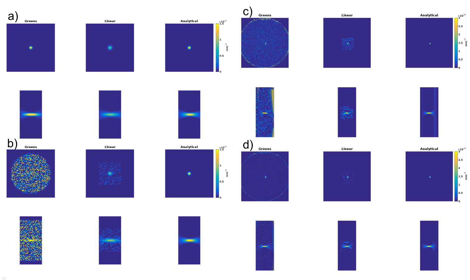
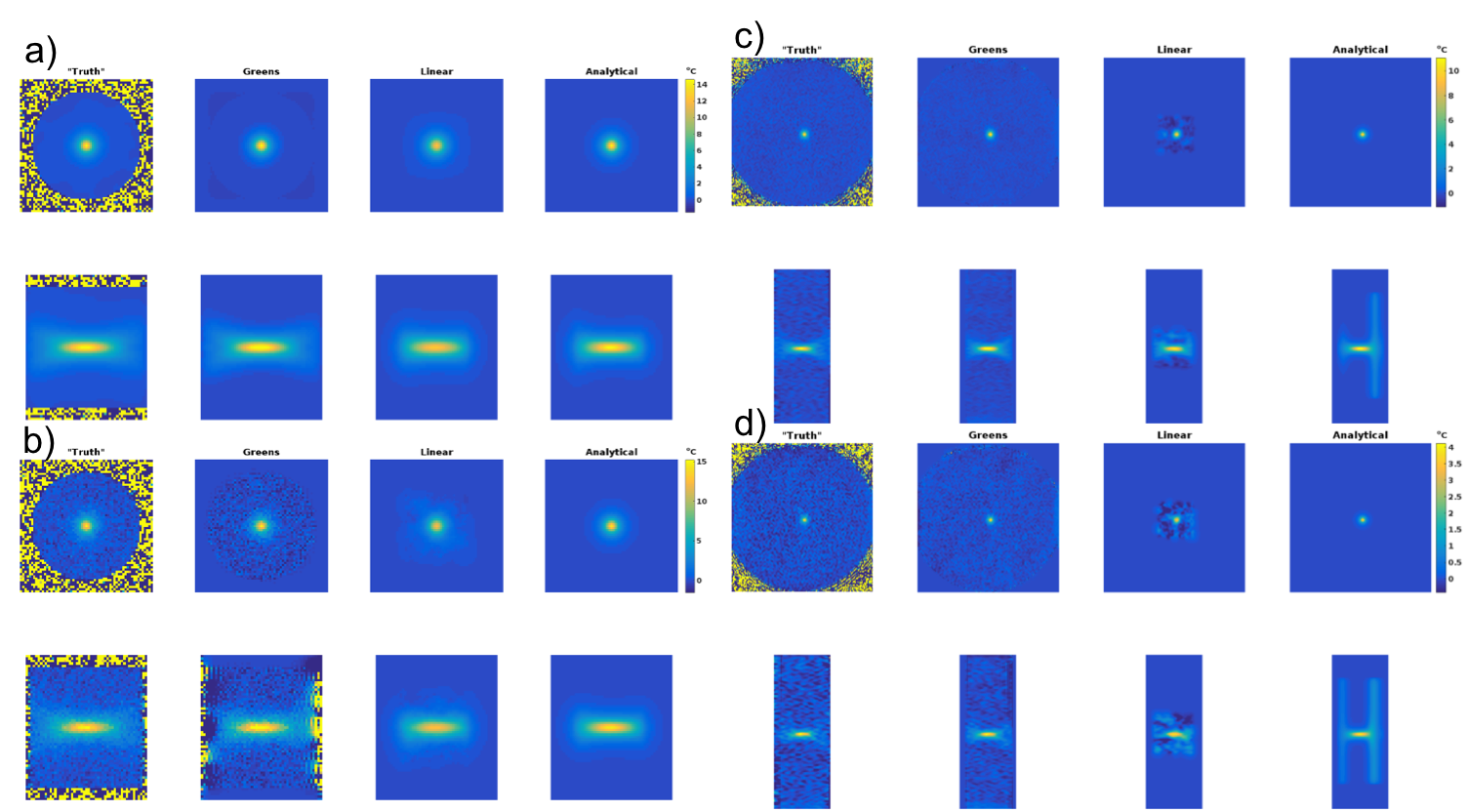
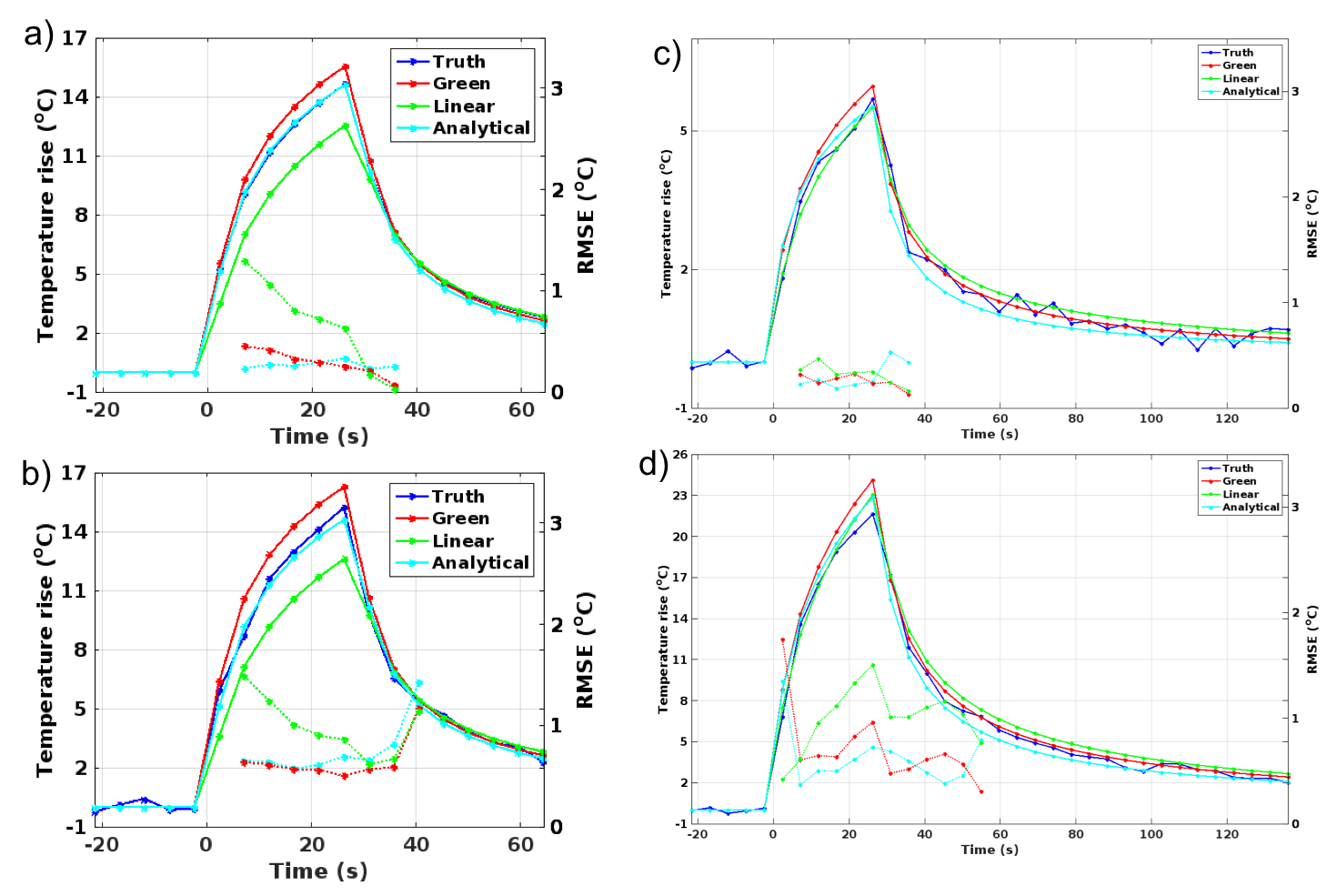
Figure 2 shows orthogonal views of Qrel for the simulation (noise-SD 0.0 and 0.4°C) and phantom (9 and 40W) experiments. Figure 3 shows corresponding orthogonal views of temperature maps obtained by inserting Qrel in the PBTE. Even though the maps from the numerical method appear noisier, they agree well with truth. Figure 4 shows line plots of temperature rise vs. time for the voxel experiencing maximum heating. The RMSE for all 5 simulated noise-levels, and all 4 phantom power levels are shown in Table 1. The time to estimate Qrel using the three methods was 3.4 s, 1363 s, and 329 s for the numerical, linear and analytical method, respectively (2.4GHz Intel Xeon compute-server, 95Gb RAM).Discussion and Conclusions
Table 2, and Figures 3 and 4, show that the accuracy of the reconstructed temperature maps from the numerical method is as good as the currently most accurate method, the analytical method, while the linear method is less accurate. This is true despite the input Q-maps from the numerical method appearing considerably noisier (Figure 2). The speed of the numerical method estimation can potentially be useful for iterative methods. Future studies will investigate adding constraints to the estimation process, to reduce noise.Acknowledgements
1 H.H. Pennes, “Analysis of tissue and arterial blood temperatures in the resting human forearm.,” J. Appl. Physiol. 1(2), 93–122 (1948).
2 R.B. Roemer, A.M. Fletcher, and T.C. Cetas, “Obtaining local SAR and blood perfusion data from temperature measurements: steady state and transient techniques compared.,” Int. J. Radiat. Oncol. Biol. Phys. 11(8), 1539–50 (1985).
3 C.R. Dillon, U. Vyas, A. Payne, D.A. Christensen, and R.B. Roemer, “An analytical solution for improved HIFU SAR estimation.,” Phys. Med. Biol. 57(14), 4527–44 (2012).
4 C.R. Dillon, N. Todd, A. Payne, D.L. Parker, D.A. Christensen, and R.B. Roemer, “Effects of MRTI sampling characteristics on estimation of HIFU SAR and tissue thermal diffusivity.,” Phys. Med. Biol. 58(20), 7291–307 (2013).
5 C.R. Dillon, G. Borasi, and A. Payne, “Analytical estimation of ultrasound properties, thermal diffusivity, and perfusion using magnetic resonance-guided focused ultrasound temperature data,” Phys. Med. Biol. 61, 923–936 (2016).
6 Y.C. Shi, D.L. Parker, and C.R. Dillon, “Sensitivity of tissue properties derived from MRgFUS temperature data to input errors and data inclusion criteria: ex vivo study in porcine muscle,” Phys. Med. Biol. 61(15), N373–N385 (2016).
7 U. Vyas and D.A. Christensen, “Extension of the angular spectrum method to calculate pressure from a spherically curved acoustic source,” J. Acoust. Soc. Am. 130(5), 2687 (2011).
8 U. Vyas and D.A. Christensen, “Ultrasound beam simulations in inhomogeneous tissue geometries using the hybrid angular spectrum method.,” IEEE Trans. Ultrason. Ferroelectr. Freq. Control 59(6), 1093–100 (2012).
9 A.I. Farrer et al., “Characterization and evaluation of tissue-mimicking gelatin phantoms for use with MRgFUS,” J. Ther. Ultrasound 3(1), 9 (2015).
10 Y. Ishihara, A. Calderon, H. Watanabe, K. Okamoto, Y. Suzuki, and K. Kuroda, “A precise and fast temperature mapping using water proton chemical shift.,” Magn. Reson. Med. 34(6), 814–23 (1995).
References
This work was supported by the Mark H. Huntsman endowed chair, and NIH grant R01 CA17278.Figures