Synopsis

We propose a new non-Cartesian sampling scheme based on a 3D cones k-space trajectory. The design framework uses a cones coordinate system that uniquely represents a point in 3D k-space with a rotation of a spiral that resides on a conic surface. The new trajectory is obtained by discretizing the proposed coordinate system. Incorporation of a variable-density spiral improves the sampling efficiency. Simulations and phantom studies demonstrate the improved efficiency of the new scheme compared to the conventional cones design.

Introduction

3D cones trajectory¹ enables highly efficient sampling compared to 3D Cartesian trajectories, which samples 3D k-space along spiral-like trajectories on a set of conic surfaces. In Gurney et al.¹, cones is proposed as a generalization of 3DPR trajectory, and its readout spokes are generated by twisting two waveforms that radiate in the radial and circumferential directions¹.

In this work, we redesign 3D cones trajectory as a generalization of a spiral trajectory. A new 3D coordinate system is derived with spirals on cones. Similar to 2DFT and 2DPR trajectories, which are discretized versions of Cartesian and polar coordinates, the new trajectory is obtained by sampling the proposed coordinate. To improve the sampling efficiency, a variable-density spiral² is adapted. The proposed design results in a trajectory with better sampling efficiency than the conventional cones trajectory.

Theory

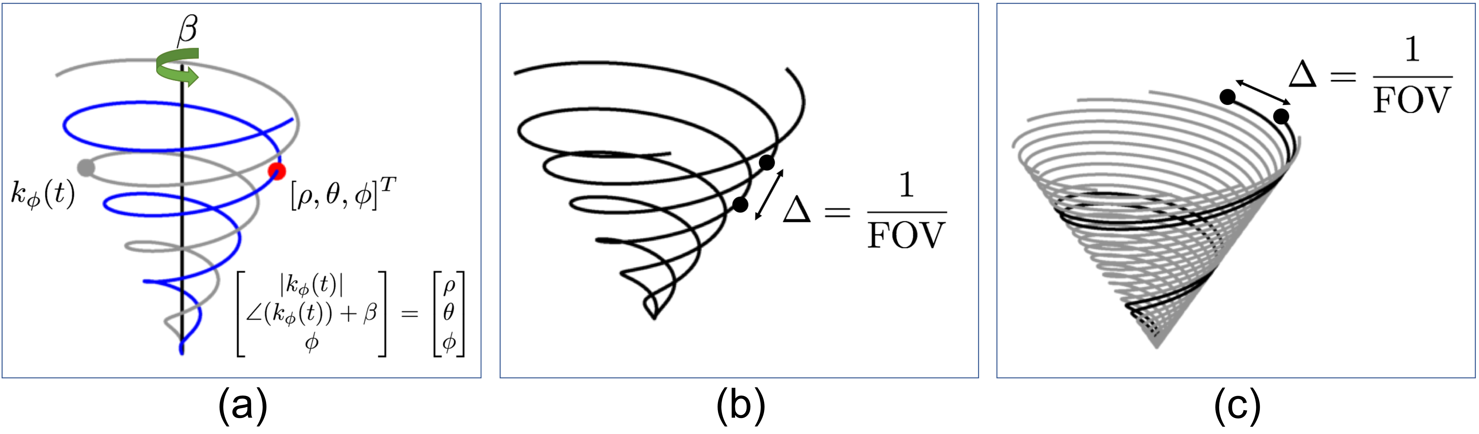
We extend a 2D spiral coordinate system³ to 3D. A point in Spherical coordinate system is represented by $$$(\rho, \theta, \phi)$$$. We define a cone as the collection of points with an identical polar angle $$$\phi$$$. The point is then on one of the cones, $$$C_\phi$$$. We consider an interleaf of a spiral $$$k_\phi(t)$$$ that resides on $$$C_\phi$$$. If we rotate $$$k_\phi(t)$$$ around the kz-axis by the angle of $$$\beta$$$, then it passes the aforementioned point if and only $$$\rho = |k_\phi(t)|$$$ and $$$\theta = \angle \left(k_\phi(t)\right) + \beta$$$ as illustrated in Figure 1(a). This leads to the following cones coordinate $$$(t, \beta, \phi)$$$:

$$\begin{align} \begin{bmatrix} \rho \\ \theta \\ \phi \\ \end{bmatrix} &= \begin{bmatrix} |\vec{k}_{\phi}(t)| \\ \angle(\vec{k}_{\phi}(t)) + \beta \\ \phi\\ \end{bmatrix}, [1] \\ \mbox{where }\vec{k}_\phi(t) &= \begin{bmatrix} r_\phi(t)\cos(\theta_\phi(t))\sin\phi \\ r_\phi(t)\sin(\theta_\phi(t))\sin\phi \\ r_\phi(t)\cos\phi\\ \end{bmatrix}.[2]\end{align} $$

The density compensation factor (DCF) is derived by the determinant of the Jacobian matrix³:

$$\frac{\gamma}{2\pi}|\vec{k}_\phi(t)|^2 |\vec{g}_\phi(t)| \cos(\vec{k}_\phi(t), \vec{g}_\phi(t)) \sin(\phi).~[3]$$

Recall that the DCF of 2D spiral is given as follows³:

$$\frac{\gamma}{2\pi}|\vec{k}_\phi(t)||\vec{g}_\phi(t)| \cos(\vec{k}_\phi(t), \vec{g}_\phi(t)).~[4]$$

A comparison between [3] and [4] suggests that the proposed approach leads to a 3D variant of the spiral trajectory.

The redesigned cones trajectory can be obtained by discretizing [1]. The discretization of $$$t$$$ and $$$\phi$$$ is done with a similar method in the conventional design^{1, 4}. The discretization of $$$\beta$$$ is equivalent to determining the number of interleaves of a spiral on each cone. FOV is then defined as the spiral trajectory (Figure 2(b)). However, FOV is determined as 3DPR in the conventional cones trajectory¹ (Figure 2(c)) even though its readout waveforms are spirals^{1, 5}. The proposed approach resolves this discrepancy, and provides a more robust way for undersampling.

To improve the sampling efficiency, we adapt the variable-density spiral² as follows:

$$\begin{align} k(t) &= \left( \frac{N_i}{2\pi L} \right)\theta(t), \mbox{ (Archimedean spiral) }\\ \Delta \theta &= \left(\frac{2\pi}{N_i}\right)L\Delta k,\\ \theta_{\mathrm{vd}}(\rho) &= \frac{2 \pi}{N_i} \int L(\rho)\mathrm{d}\rho, \label{eq:vd_spiral_theta} [5]\\ k_{\mathrm{vd}}(\rho) &= \rho \cdot \theta_{\mathrm{vd}}(\rho), \mbox{ (Variable-density spiral)}\end{align}$$

where $$$N_i$$$ denotes the number of interleaves, $$$L(\rho)$$$ represents the effective FOV along the radial distance $$$\rho$$$. The sampling density can be tuned by substituting $$$r_\phi(t)$$$ and $$$\theta_\phi(t)$$$ in [2] with $$$\rho$$$ and $$$\theta_{\mathrm{vd}}(\rho)$$$ in [5].

Methods

For the simulation study, a numerical phantom was acquired from MRXCAT⁶, and cropped to the size of (28,28,14)-cm. Simulated data were generated and reconstructed by inverse and forward 3D griddings.

A GE 1.5T scanner (Waukesha, WI) with an 8-channel cardiac coil was used for the phantom study. An ATR-SSFP sequence⁷ was prescribed with following scan parameters: TE/TR₁/TR₂ = 0.57/1.15/4.55-ms, 70-degree flip angle, and 2.8-ms duration for readout waveforms.

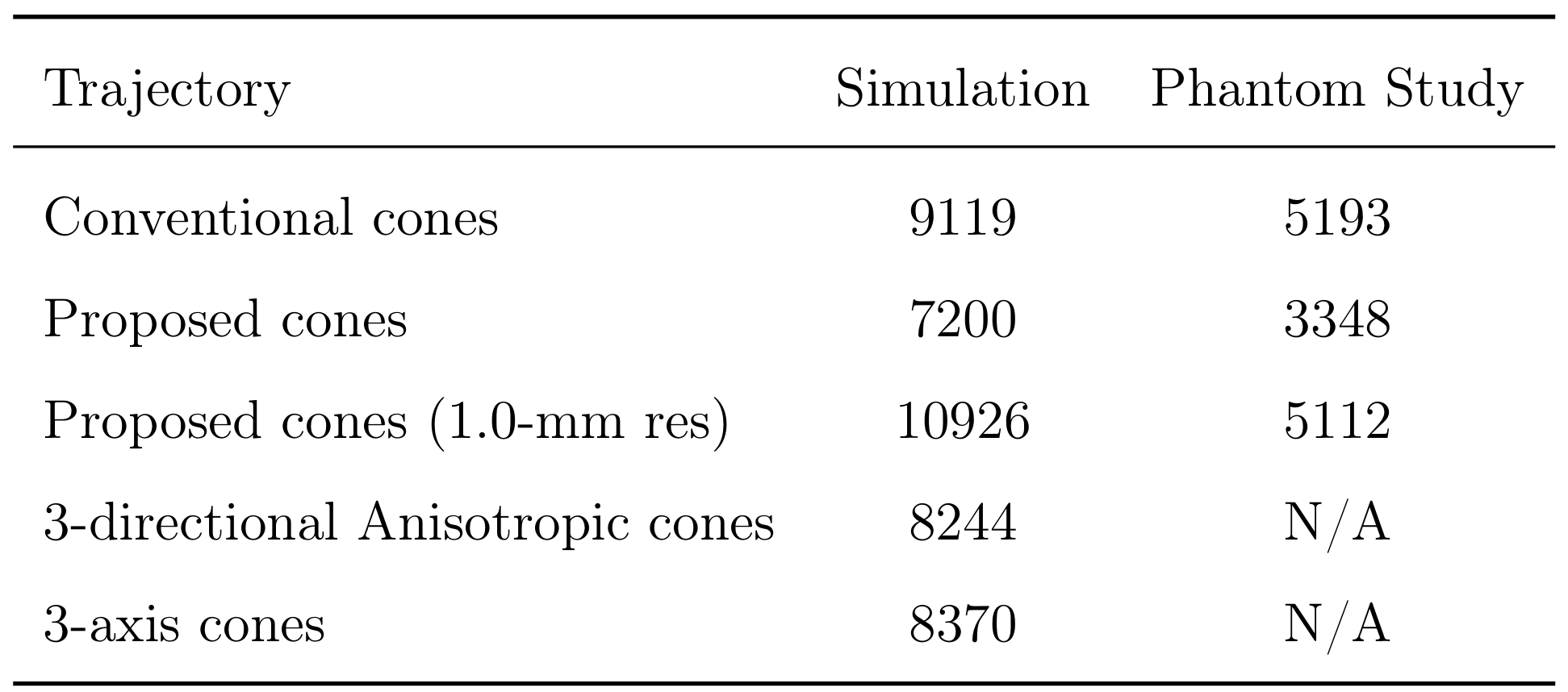
The FOVs were (28,28,14)-cm, and (16,16,14)-cm for the simulation and phantom studies, respectively. The default resolution was isotropic 1.2-mm. To match the numbers of readouts, a finer resolution of 1.0-mm was tested for the proposed trajectory. The number of readouts are listed in Table 1. ESPIRiT⁸ was used in the phantom study.

Results

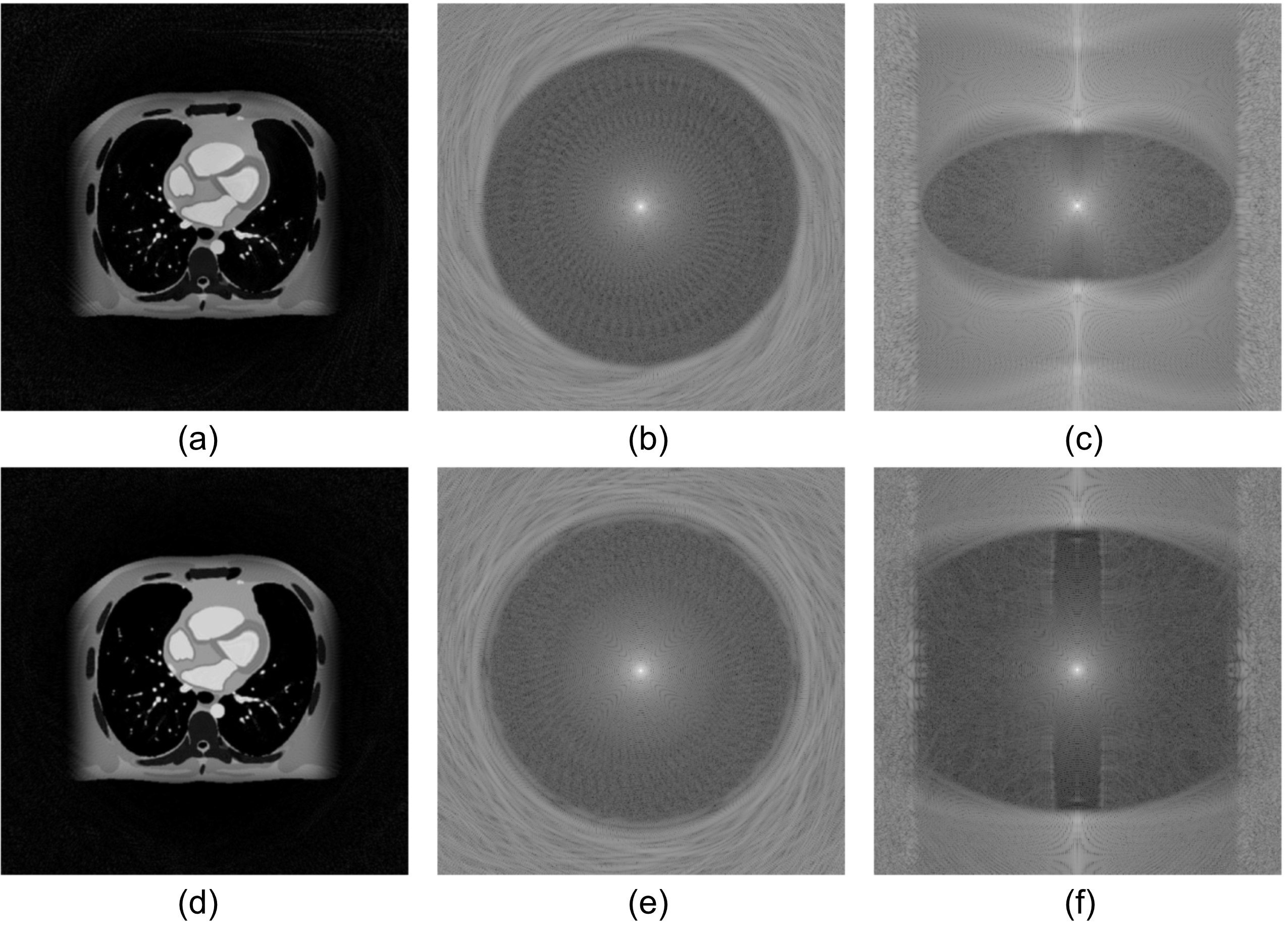
The reconstructed slices in the simulation are illustrated in Figure 2. We can observe little aliasing artifact within the FOV in Figure 2(a), despite the proposed trajectory using 78.96% the number of readouts as compared to conventional cones. The redefined cones trajectory showed more defined FOV as illustrated in Figure 2(b, c) compared to Figure 2(e, f), which allows a significant reduction in the scan time.

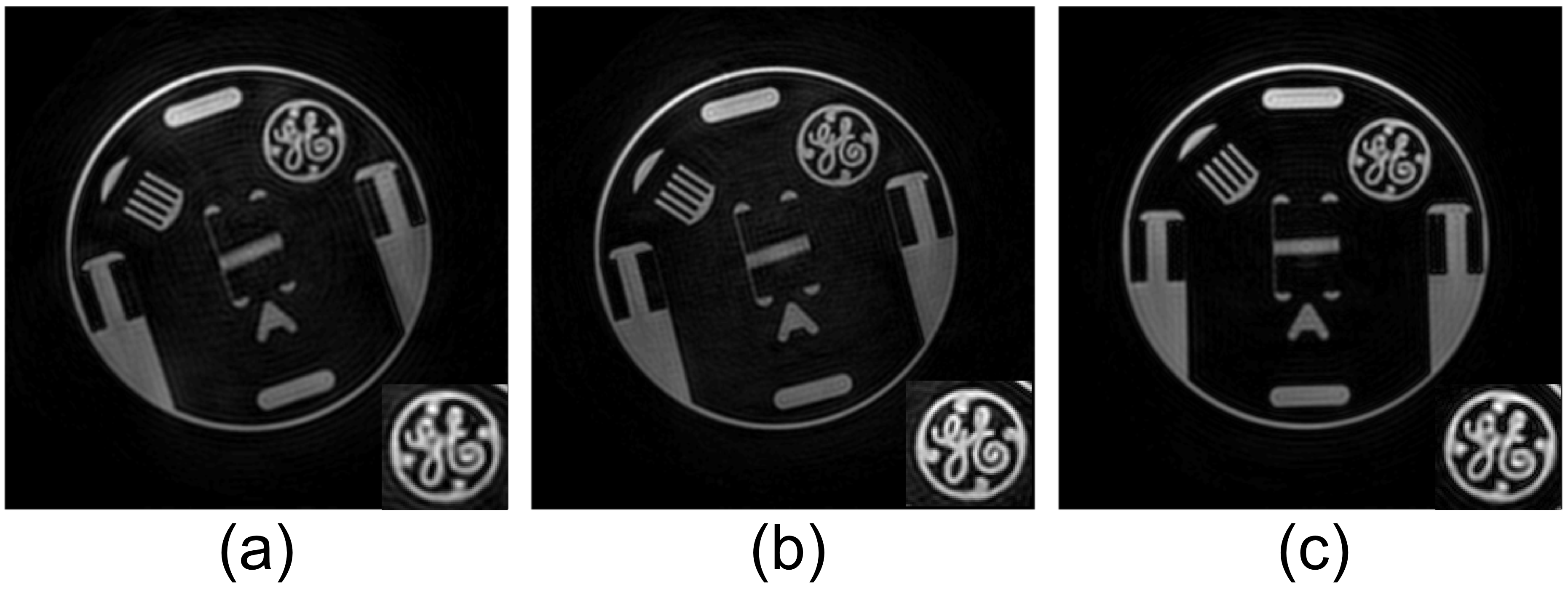
The phantom image with the proposed method (Figure 3(a)) compares well with the conventional cones method (Figure 3(c)), despite using 64.47% the number of readouts. When the number of readouts are matched, the proposed trajectory enables finer resolution, as illustrated in Figure 3(b).

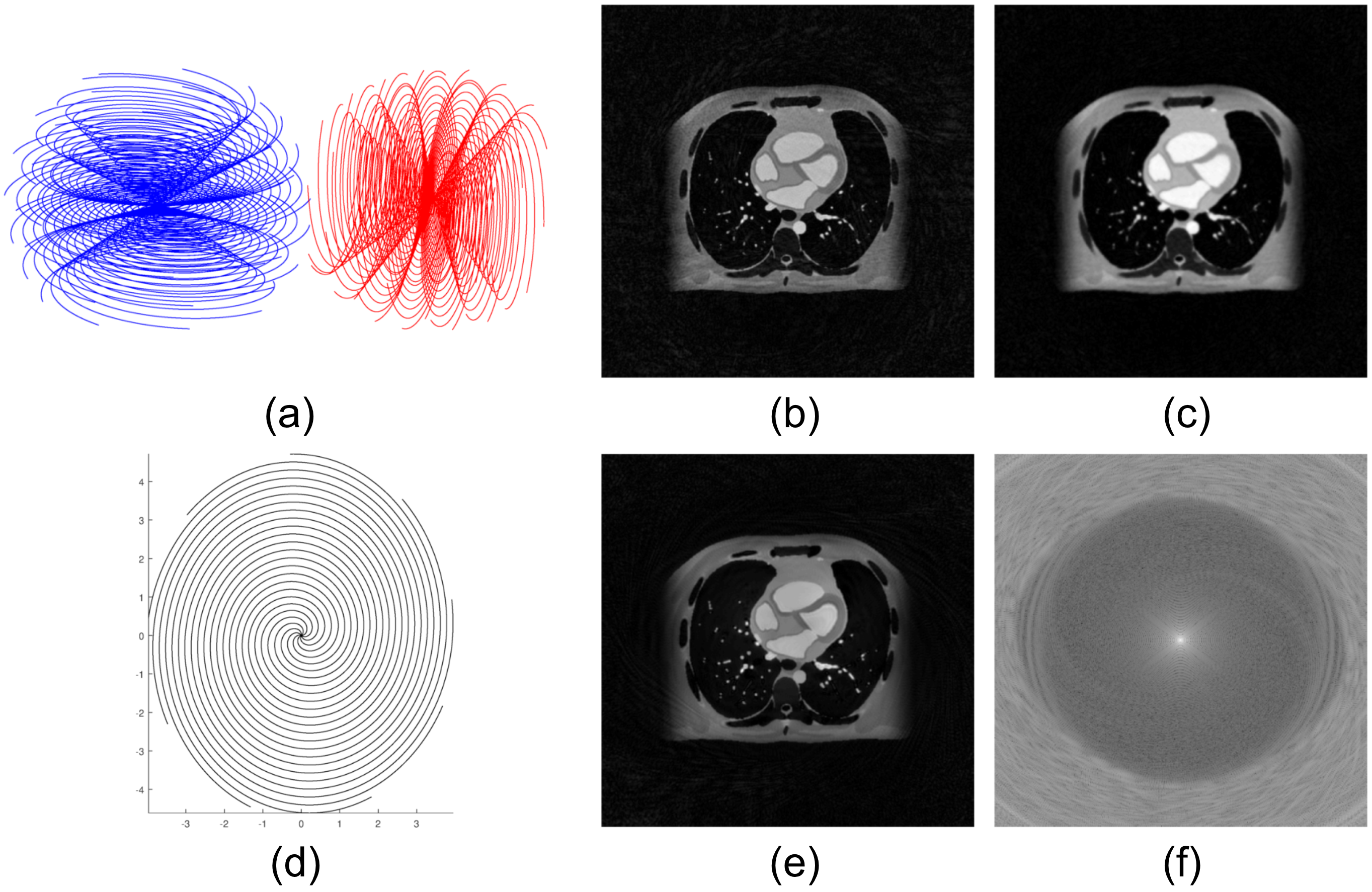
Studies on extensions of the proposed approach are illustrated in Figure 4.

Conclusion

Acknowledgements

References

1. P. T. Gurney, B. A. Hargreaves, and D. G. Nishimura, "Design and analysis of a practical 3D cones trajectory,” Magnetic resonance in medicine, vol. 55, no. 3, pp. 575–582, 2006.

2. J. H. Lee, B. A. Hargreaves, B. S. Hu, and D. G. Nishimura, “Fast 3D imaging using variable-density spiral trajectories with applications to limb perfusion,” Magnetic resonance in medicine, vol. 50, no. 6, pp. 1276–1285, 2003.

3. R. D. Hoge, R. K. Kwan, and G. Bruce Pike, “Density compensation functions for spiral MRI,” Magnetic Resonance in Medicine, vol. 38, no. 1, pp. 117–128, 1997.

4. P. E. Larson, P. T. Gurney, and D. G. Nishimura, “Anisotropic field-of-views in radial imaging,” IEEE transactions on medical imaging, vol. 27, no. 1, pp. 47–57, 2008.

5. N. O. Addy, R. R. Ingle, H. H. Wu, B. S. Hu, and D. G. Nishimura, “High-resolution variable-density 3D cones coronary MRA,” Magnetic resonance in medicine, vol. 74, no. 3, pp. 614–621, 2015.

6. L. Wissmann, C. Santelli, W. P. Segars, and S. Kozerke, “MRXCAT: Realistic numerical phantoms for cardiovascular magnetic resonance,” Journal of Cardiovascular Magnetic Resonance, vol. 16, no. 1, p. 63, 2014.

7. H. H. Wu, P. T. Gurney, B. S. Hu, D. G. Nishimura, and M. V. McConnell, "Free-breathing multiphase whole-heart coronary MR angiography using image-based navigators and three-dimensional cones imaging," Magnetic resonance in medicine, vol. 69, no. 4, pp. 1083–1093, 2013.

8. M. Uecker, P. Lai, M. J. Murphy, P. Virtue, M. Elad, J. M. Pauly, S. S. Vasanawala, and M. Lustig, "ESPIRiT—an eigenvalue approach to autocalibrating parallel MRI: where SENSE meets GRAPPA," Magnetic resonance in medicine, vol. 71, no. 3, pp. 990–1001, 2014.

9. J. G. Pipe, N. R. Zwart, E. A. Aboussouan, R. K. Robison, A. Devaraj, and K. O. Johnson, “A new design and rationale for 3d orthogonally oversampled k-space trajectories,” Magnetic resonance in medicine, vol. 66, no. 5, pp. 1303–1311, 2011.

10. N. R. Zwart, K. O. Johnson, and J. G. Pipe, “Efficient sample density estimation by combining gridding and an optimized kernel,” Magnetic resonance in medicine, vol. 67, no. 3, pp. 701–710, 2012

11. K. F. King, “Spiral scanning with anisotropic field of view,” Magnetic resonance in medicine, vol. 39, no. 3, pp. 448–456, 1998.