4147
APIR4EMC: Autocalibrated Parallel Imaging Reconstruction for Extended Multi-Contrast Imaging1Departments of Medical Informatics, Erasmus Medical Center, Rotterdam, Netherlands, 2Departments of Radiology and Nuclear Medicine, Erasmus Medical Center, Rotterdam, Netherlands
Synopsis
Multi-contrast images of the same region are routinely acquired in clinical MRI. This abstract proposes a fast reconstruction method for multi-contrast imaging: Autocalibrated Parallel Imaging Reconstruction for Extended Multi-Contrast (APIR4EMC). Unlike conventional parallel imaging (GRAPPA) which reconstructs the image for individual contrast, APIR4EMC additionally includes the inter-contrast signals in the prediction of unsampled positions in the k-space of each contrast and simultaneously reconstructs images for all contrasts. Experiments show significant improvement of APIR4EMC compared to conventional parallel imaging in terms of artifacts and SNR.
Introduction
Images showing different contrasts of the same region are routinely acquired in clinical magnetic resonance imaging (MRI). To accelerate the imaging, parallel imaging (e.g. GRAPPA) is commonly used. It uses differences in sensitivity profile among channels of multi-channel coils to restore unsampled k-space positions. We propose to additionally use the correlation across different contrasts in our Autocalibrated Parallel Imaging Reconstruction for Extended Multi-Contrast (APIR4EMC) method.Methods
In [1] a GRAPPA based method, APIR4GRASE, was proposed for the GRASE sequence. It compensates differences between gradient echoes and spin echoes automatically by treating these contrasts as additional coil channels in the GRAPPA/APIR reconstruction. In this work we extend this method to arbitrary contrasts for multi-contrast imaging and propose APIR4EMC, which encodes the correlation across multiple contrasts along with the coil sensitivity into the GRAPPA reconstruction kernel. This enables all contrasts to contribute to the reconstruction of each individual contrast.
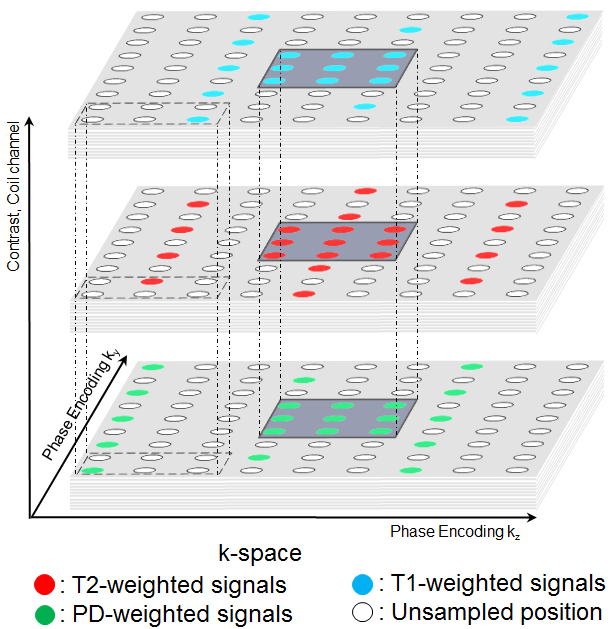
Similar to GRAPPA, APIR4EMC regularly subsamples the k-space of each contrast. Autocalibration signals (ACS) are acquired from a small fully sampled k-space center region. Unlike coil channels, different contrasts can shift k-space subsampling patterns with respect to each other (see Figure 1).
Variable flip angle Fast Spin Echo (FSE) [2] enables multi-contrast imaging by changing TR, TE and/or preparation pulses. Additionally, as the contrast evolves along the echo train (ET), the ET may be separated into parts differing in contrast weighting. By distributing each ET part radially in k-space [3], its contrast is dominated by the contrast at the start of that part.
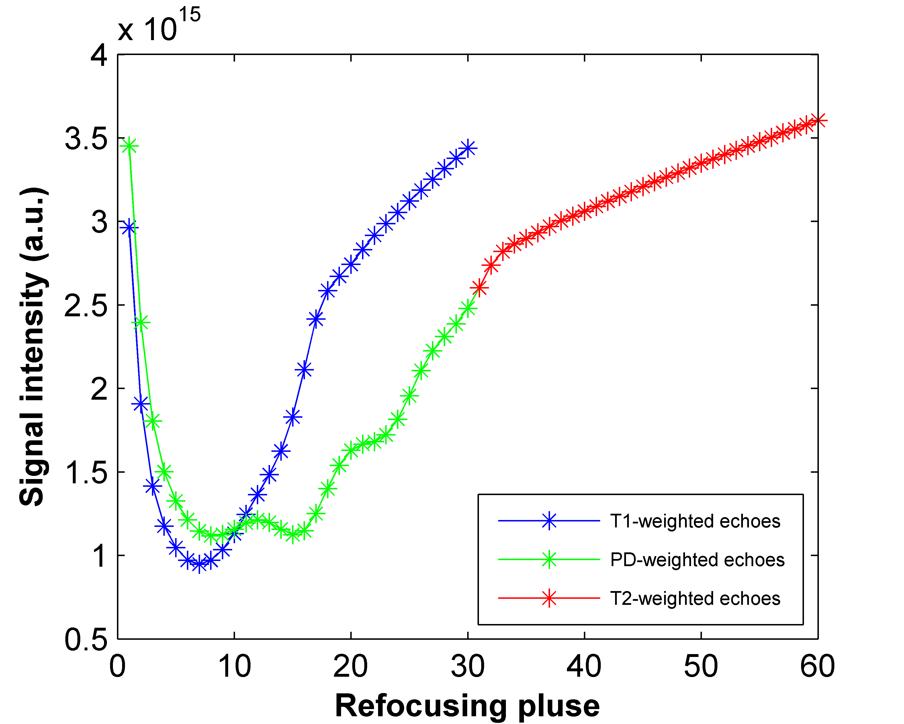
Nevertheless, the signal evolution along the ET may differ among contrasts. This may create artifacts as the contrast correlation encoded in the GRAPPA kernel is computed from the ACS region filled by a small part of the ET. To compensate the modulation, APIR4EMC acquires an additional zero-phase-encoded echo train as reference and divides each echo of each contrast by the norm of the corresponding reference echo before the reconstruction.
Experiments
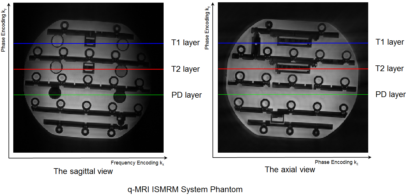
To evaluate the performance of the method, multi-contrast weighted images were acquired. Specifically, two variable flip angle [2] 3D FSE acquisitions were used to obtain T1-, T2- and PD- weighted images of the q-MRI ISMRM system phantom [4] on a 3T GE (MR750) scanner using an 8-channel head coil. Common settings: $$$matrix=256\times256\times256$$$, $$$FOV=230\times230\times230mm^3$$$, $$$BW/pixel=83.33kHz$$$, and Radial trajectory [3]. For T1-weighted contrast, $$$TR/ESP/ETL=500ms/3.872ms/30$$$, while for T2/PD-weighted, $$$TR/ESP/ETL=2000ms/3.872ms/60$$$. The first and the last 30 echoes were separately placed in PD- and T2 weighted k-spaces, respectively (see Figure 4).
We used a subsampling factor of $$$2\times3$$$ in two phase encoding (PE) dimensions in a CAIPIRINHA pattern [5] with a $$$25\times25$$$ calibration region (see Figure 1). The GRAPPA image was reconstructed on each individual contrast with the convolution kernel size of $$$5(PE1)\times5(PE2)\times8(channel)$$$. APIR4Multicontrast images were reconstructed simultaneously for three contrasts with the kernel size of $$$5(PE1)\times5(PE2)\times8(channel)\times3(contrast)$$$. As reference we acquired full k-spaces for each contrast. Scan time was 16 min for the complete subsampled acquisition, and 91 min for the reference.
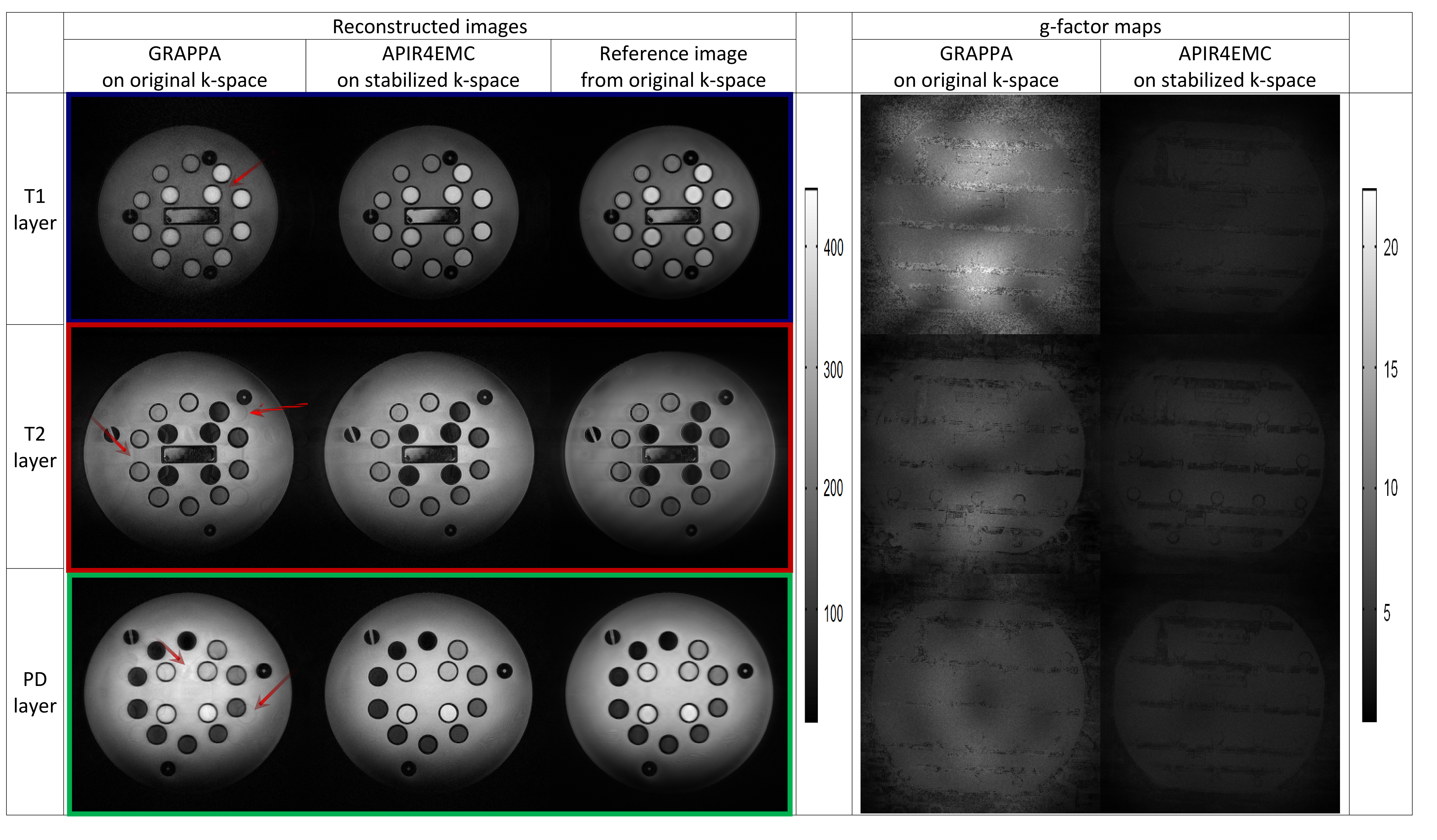
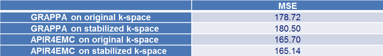
As quantitative measure, the MSE of APIR4EMC and GRAPPA reconstructed images to the full reference image, excluding a small region containing an air bubble, is computed. The g-factor is computed with 300 pseudo replicas [6].
Results and Discussion
The reconstructed images and g-factor maps are shown in Figure 3. Compared to the GRAPPA images where a lot of artifacts exist, APIR4EMC shows lower noise amplification and fewer artifacts in each contrast image. Figure 4 presents the signal evolution for the three contrasts. By normalizing the signal envelope into the same steady state, APIR4EMC did not suffer from the scaling difference along the envelope between different contrasts. As GRAPPA is single contrast, it does not have this problem. Additional results (images not shown) demonstrated that the stabilization procedure reduced the artifacts for APIR4EMC while for GRAPPA the difference is negligible, though it helped slightly reduce apparent blurring. The MSE in Figure 5 confirms these qualitative observations.Conclusion
The results show that the selected acceleration factor of 6 using GRAPPA for each individual contrast exceeds the possibilities of the used 8 channel head coil. By including multi-contrast data into the reconstruction process, APIR4EMC is able to reduce artifacts and noise amplification for each contrast compared to GRAPPA under the sample subsampling factor. Thus, APIR4EMC enables increased acceleration capability for multiple contrasts acquisitions.Acknowledgements
No acknowledgement found.References
1. Zhang C, Cristobal-Huerta A, Hernández Tamames J A, et al, A new pattern for Autocalibrated Parallel Imaging Reconstruction for GRASE: APIR4GRASE, Proceeding ISMRM, 2017, 5162.
2. Busse R F, Hariharan H, Vu A, et al. Fast spin echo sequences with very long echo trains: design of variable refocusing flip angle schedules and generation of clinical T2 contrast[J]. Magnetic Resonance in Medicine, 2006, 55(5): 1030-1037.
3. Busse R F, Brau A, Vu A, et al. Effects of refocusing flip angle modulation and view ordering in 3D fast spin echo[J]. Magnetic Resonance in Medicine, 2008, 60(3): 640-649.
4. http://www.hpd-online.com/system-phantom.php
5. Breuer F A, Blaimer M, Mueller M F, et al. Controlled aliasing in volumetric parallel imaging (2D CAIPIRINHA)[J]. Magnetic Resonance in Medicine, 2006, 55(3): 549-556.
6. Robson P M, Grant A K, Madhuranthakam A J, et al. Comprehensive quantification of signal‐to‐noise ratio and g‐factor for image‐based and k‐space‐based parallel imaging reconstructions[J]. Magnetic Resonance in Medicine, 2008, 60(4): 895-907.
Figures