4102
Novel and Efficient Generation of Diffeomorphic Motion Phantom1Parallel Computing Lab, Intel Corporation, Hillsboro, OR, United States, 2Department of Radiology, Massachusetts General Hospital and Harvard Medical School, Boston, MA, United States, 3The Center for Clinical Data Science, Massachusetts General Hospital and Brigham and Women’s Hospital, Boston, MA, United States
Synopsis
Dealing with motion artifacts is a fundamental preprocessing step in magnetic resonance imaging (MRI). In this work, we present three novel methods to generate MRI phantoms for diffeomorphic motion which can be used to validate motion correction algorithms. Previous research efforts for diffeomorphic motion generation, employ a brute force approach in which random pixel/voxel displacements are repeatedly generated until a topologically valid displacement is found. Such methods are not only time consuming but also doesn’t guarantee a valid displacement. Our approach algorithmically ensures that the topological properties are always maintained resulting in guaranteed diffeomorphic motion with much faster runtime.
INTRODUCTION
The acquisition time of Magnetic resonance imaging (MRI) makes it susceptible to motion artifacts [2]. Various motion correction algorithms have been proposed [3,4,5], synthetically generated motion phantom is a solid way to validate and evaluate such algorithms.
Previous efforts to generate diffeomorphic motion phantoms[1] involve repeatedly generating random voxel displacements until one that satisfies topological properties is found. Such brute force approaches are cumbersome and doesn’t guarantee a valid diffeomorphic motion in a given amount of time. In this work, we propose three novel methods to efficiently generate diffeomorphic motion phantom which algorithmically ensure topology preservation.
METHODS
Suppose $$$s_1<s_2<s_3…<s_n$$$ are the coordinates of each pixel along a given axis before motion, and the maximum allowed displacement is $$$d_{max}$$$. After motion injection, each of $$$s_i$$$ is transformed to target coordinates $$$t_i$$$. To preserve topology, $$$t_1<t_2<t_3…<t_n$$$ needs to be guaranteed.
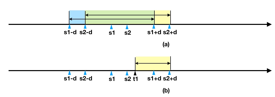
Algorithm 1: Sequential Method (SM). To preserve topology, this method takes into account both $$$d_{max}$$$ and the displacement of neighboring pixel (Figure 1) to decide the displacement of a pixel. SM involves following steps:
- Select the size of the generator kernel (e.g. [2,5,5]) which is some fraction of the image size.
- For each pixel in the kernel, randomly draw $$$p_i\in (0,1]$$$ which signifies the percentage location within the topologically valid displacement range defined in step 4.
- Upsampling the drawn values to original image size with interpolation, followed by Gaussian smoothing and re-scaling it back to $$$(0,1]$$$ range in order to ensure smoothness of the displacement field.
- For the first pixel in each axis, randomly draw its target coordinate, from $$$d\in[s_1-d_{max},s_1+d_{max}]$$$. For all other pixels the topologically valid target coordinates can be drawn from $$$t_i\in[max(t_1,t_{i-1}-d_{max}), s_i+d_{max}]$$$ with range $$$r_i=s_i+d_{max}-max(t_1,t_{i-1}-d_{max})$$$. This ensures that no two pixels overlap with each other after motion.
- The target coordinates for each pixel are calculated using the percentage location in the valid range, $$$t_i=p_i*r_i$$$.
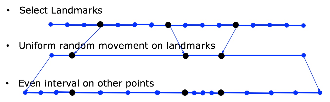
Algorithm 2: Landmark Method(LM). The motivation behind this method is that similar type of tissues tend to have similar degree of displacement. The LM (Figure 2) involve following steps:
- Select $$$m$$$ landmark pixels $$$l_i\in[s_1,s_1,..s_n]$$$, that decides how many different types of tissues to be model.
- For each landmark pixel $$$l_i$$$, randomly draw its target coordinates from $$$tl_i\in [l_i-d_{max}, l_i+d_{max}]$$$
- For each pixel between two landmarks, their target coordinates are evenly distributed between the corresponding landmarks.
- For pixels topologically before the first landmark, the target coordinates evenly distributed between the minimum valid coordinate and the first landmark i.e., $$$[s_1-d_{max},tl_1]$$$.
- For pixels topologically after the last landmark, the target coordinates are evenly distributed between the last landmark and the maximum valid coordinate i.e., $$$[tl_m,s_n+d_{max}]$$$. Hence this method ensures that the topological properties among landmark pixels and pixels in between the landmarks are maintained after motion injection with a coordinated similar degree of displacement among the intra landmark pixels.
- Finally the displacement field is calculated by $$$d_i=t_i-s_i$$$ followed by applying a Gaussian smoothing and rescaling to $$$[-d_{max},d_{max}]$$$ range.
Algorithm 3: Cumulative Sum Method(CSM). Methods discussed so far generates displacement values that preserves the initial topology and hence adds dependencies in their calculation, rendering them computationally intensive. CSM, rather than using displacement values, makes sure that the distance between two consecutive pixels is always greater than zero:
- Select the size of the generator kernel.
- For the first pixel in each axis, randomly draw its target coordinate from $$$t_1\in[s_1-d_{max},s_1+d_{max}]$$$.
- For all other pixels, randomly draw its distance $$$r_i$$$ from the previous pixel, from $$$r_i\in(0, d_{max}]$$$.
- Upsampling the drawn distance to the original image size with bilinear interpolation followed by Gaussian smoothing.
- For all but the first pixels, target coordinate is calculated using $$$t_i=t_1+\sum_2^ir_i$$$, where $$$i>1$$$. This cumulative sum step ensures that the topological order is maintained.
RESULTS AND DISCUSSION
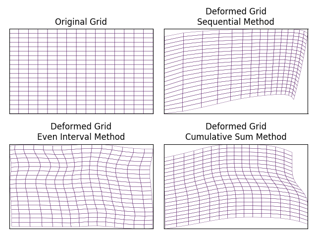
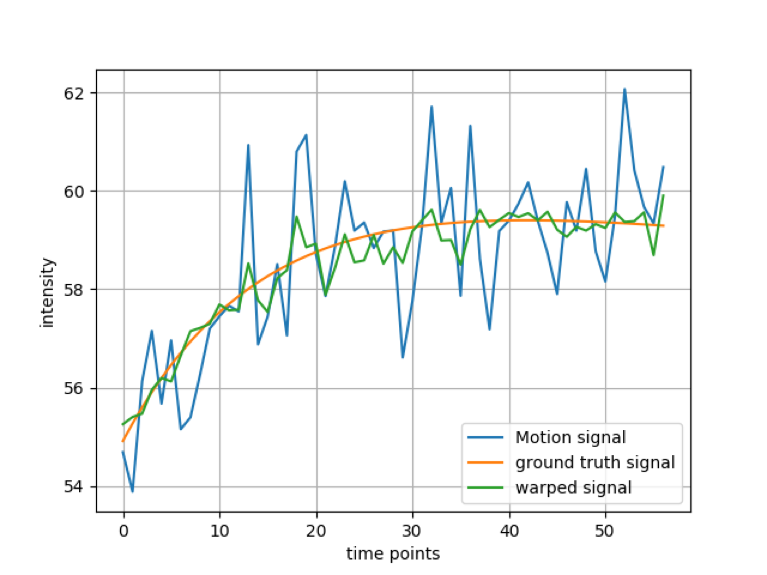
Figure 3 shows the experimental configurations and runtime of different methods. CSM is computationally fastest among the proposed methods. In SM, $$$r_{i+1}$$$ is calculated after $$$r_i$$$ and LM depends on landmarks to decide other pixels’ target coordinates, which makes them both slower than CSM. Figure 4 shows the generated deformation fields from proposed methods. Compared to the brute force approach which does not guarantee valid diffeomorphic motion, all of our methods algorithmically ensures that. Naturally, the generated phantom diffeomorphic motion can be used to verify and evaluate different registration/motion correction algorithms. Figure 5 shows an example of registration result by using diffeomorphic motion generated by LM.CONCLUSION
We have proposed three novel methods to efficiently generate diffeomorphic motion guaranteeing topology preservation. CSM is the fastest among them and LM takes spatial similarity and tissue properties into account. These methods can be used for generating diffeomorphic motion phantoms and to evaluate different registration algorithms.Acknowledgements
No acknowledgement found.References
- M. Bhushan, J. Schnabel, L. Risser, M. Heinrich, J. Brady, and M. Jenkinson, “Motion correction and parameter estimation in dcemri sequences: Application to colorectal cancer,” in Proceedings of Medical Image Computing and Computer-Assisted Intervention - MICCAI 2011, 2011, pp. 476–483.
- Tavallaei MA, Johnson PM, Liu J, Drangova M. Design and evaluation of an MRI-compatible linear motion stage. Med Phys. 2016;43:62–71.
- T. Vercauteren, L. Grady, X. Pennec, N. Ayache, and F. Cheriet, “Diffeomorphic demons: Efficient non-parametric image registration,” NeuroImage, vol. 45, pp. 61–72, 2009.
- T. Vercauteren, X. Pennec, A. Perchant, and N. Ayache, “Symmetric log-domain diffeomorphic registration: A demons-based approach.” in Proceedings of Medical Image Computing and Computer-Assisted Inter- vention - MICCAI 2011, vol. 5241, 2008, pp. 754–761.
- H. Lombaert, L. Grady, X. Pennec, N. Ayache, and F. Cheriet, “Spectral log-demons: Diffeomorphic image registration with very large deforma- tions,” International Journal of Computer Vision, vol. 107, pp. 254–271, 2014.
Figures