4097
Machine learning algorithms for detection of motion artifacts: a general approach1Department of Biomedical Magnetic Resonance, Otto-von-Guericke University, Magdeburg, Magdeburg, Germany, 2German Center for Neurodegenerative Diseases, Magdeburg, Germany, 3Center for Behavioral Brain Sciences, Magdeburg, Germany, 4Leibniz Institute for Neurobiology, Magdeburg, Germany
Synopsis
Despite all the developments to overcome MRI motion artifacts, there are still open questions. When do we need to repeat a scan? Is the image quality sufficient for segmentation or to make a diagnosis? Is the motion correction working properly? Independent of the type of image acquired (structural, diffusion, functional, etc.), machine learning algorithms can detect automatically motion artifacts and provide feedback in real time. In this work different machine learning algorithms have been tested to detect motion artifacts in synthetic and in vivo data.
INTRODUCTION
MRI scans often last several minutes during which subject motion can occur. This motion can create image artifacts, such as blurring and ghosting, and reduce the image quality. Depending on the level of image corruption, images might be usable or reacquisition may be required. The main goal of this work was to investigate the capability of different basic machine learning algorithms1 to classify image quality of simulated and of in-vivo data acquired at ultra-high field MRI.METHODS
Motion detection with machine learning was tested for three synthesized datasets. The first dataset was created from a 2D Shepp-Logan phantom (256x256 pixels): 10000 images without motion artifacts, and 10000 images containing a known level of motion artifacts, (see Fig.1, column (a)). The second dataset created from a 3D Shepp-Logan phantom (256x256x256 pixels): 12800 images without motion artifacts, 50 volumes with different orientation and position in 3D space and the same number of volumes with motion artifacts, (see Fig.2, column(b)). The last synthetic dataset consisted of 3D T1-weighted (T1-w) brain images, resolution 1.5 mm isotropic, 128x128x128 voxels, 100 volumes (12800 images) were generated without and with motion artifacts (in total 25600 images; see Fig.1, column (c)). All synthesized data included background noise and field inhomogeneities. For the in vivo data, 21 healthy subjects, after written consent, were scanned at 7T (Siemens, Erlangen, Germany) with a 32-channel head coil (Nova Medical, Wilmington, USA), using 3D-MPRAGE with prospective motion correction functionality2 (PMC): T1-w images, full brain acquisition, 0.45x0.45x0.45 mm, TR/TE/TI 2820/2.82/1050 ms, FA 5°; and were asked not to move. For tracking rigid body subject motion, a single in-bore camera tracked the position of a marker (MT384ib, Metria Innovation Inc., Milwaukee, WI,USA), which was rigidly attached to the subject’s upper jaw with an individually manufactured mouthpiece. Every subject was scanned with and without PMC, (order of PMC ON – PMC OFF was randomized). Additionally, 3 subjects were asked to follow with their head a determined motion pattern during scanning (done with and without PMC). In total 48 volumes (19968 images, 416 slices for each volume) were acquired, examples are shown in Fig. 2 (c). For all images several features were extracted, for example: mean, variance, standard deviation, texture features4 calculated from the gray level co-occurrence matrix (glcm) and features related to the edges (all the data are available at: https://github.com/sarcDV/phantom_data). Support Vector Machine (SVM), Logistic Regression (LR) and Nearest Neighbors (NN) were used to classify the extracted features from the images1. The synthetic data sets were split randomly into train and test subsets (70%, 30%) for all processing. Also others splitting ratios train/test subsets were tested, (60%, 40%), (50%, 50%).RESULTS
The synthesized 2D dataset was classified with the SVM algorithm using the image mean and Scharr’s operator3 (edge detector) with 4 different kernels (see Fig. 3). For both 3D synthetic datasets LR was used. This linear model allows to differentiate the data with decision boundaries as shown in Fig. 4 a),b). For the in-vivo dataset LR and NN classification were used. Fig. 5 b) shows the NN classification applied to the group of features: glcm-energy1 (texture analysis4) vs. Scharr’s characteristic.DISCUSSION
The results show that it is possible to detect motion artifacts without using complex approaches such as neural networks. In particular, synthetic data could be classified using simple features (mean and variance). This is due to the fact that the synthesized images could be labelled exactly (0= no motion artifacts, 1= motion artifacts) and this led to have a clear separation into 2 classes. For the in-vivo dataset, all acquisitions acquired after asking the subjects not to move (42 volumes), were labelled with 0, no motion artifacts. This assumption was based on a preliminary subjective image quality assessment. The data classified with the motion artifacts are only 6 volumes in total, consequently the final training dataset for the in-vivo test is unbalanced. But, it is still possible to observe with LR analysis a clear separation between the 2 groups motion/no motion artifacts (see Fig. 5).
Acknowledgements
This work was supported by the Initial Training Network, HiMR, funded by the FP7 Marie Curie Actions of the European Commission, grant number FP7-PEOPLE-2012-ITN-316716, and by the NIH, grant number 1R01-DA021146.References
1. Ethem Alpaydin. 2010. Introduction to Machine Learning (2nd ed.). The MIT Press.
2. Stucht D, et al. Highest Resolution In Vivo Human Brain MRI Using Prospective Motion Correction. PloS one 10, e0133921 (2015).
3. B. Jaehne, H. Scharr, and S. Koerkel. Principles of filter design. In Handbook of Computer Vision and Applications. Academic Press, 1999.
4. Robert M. Haralick, K. Shanmugam, and Its'hak Dinstein, "Textural Features for Image Classification", IEEE Transactions on Systems, Man, and Cybernetics, 1973, SMC-3 (6): 610–621.
Figures
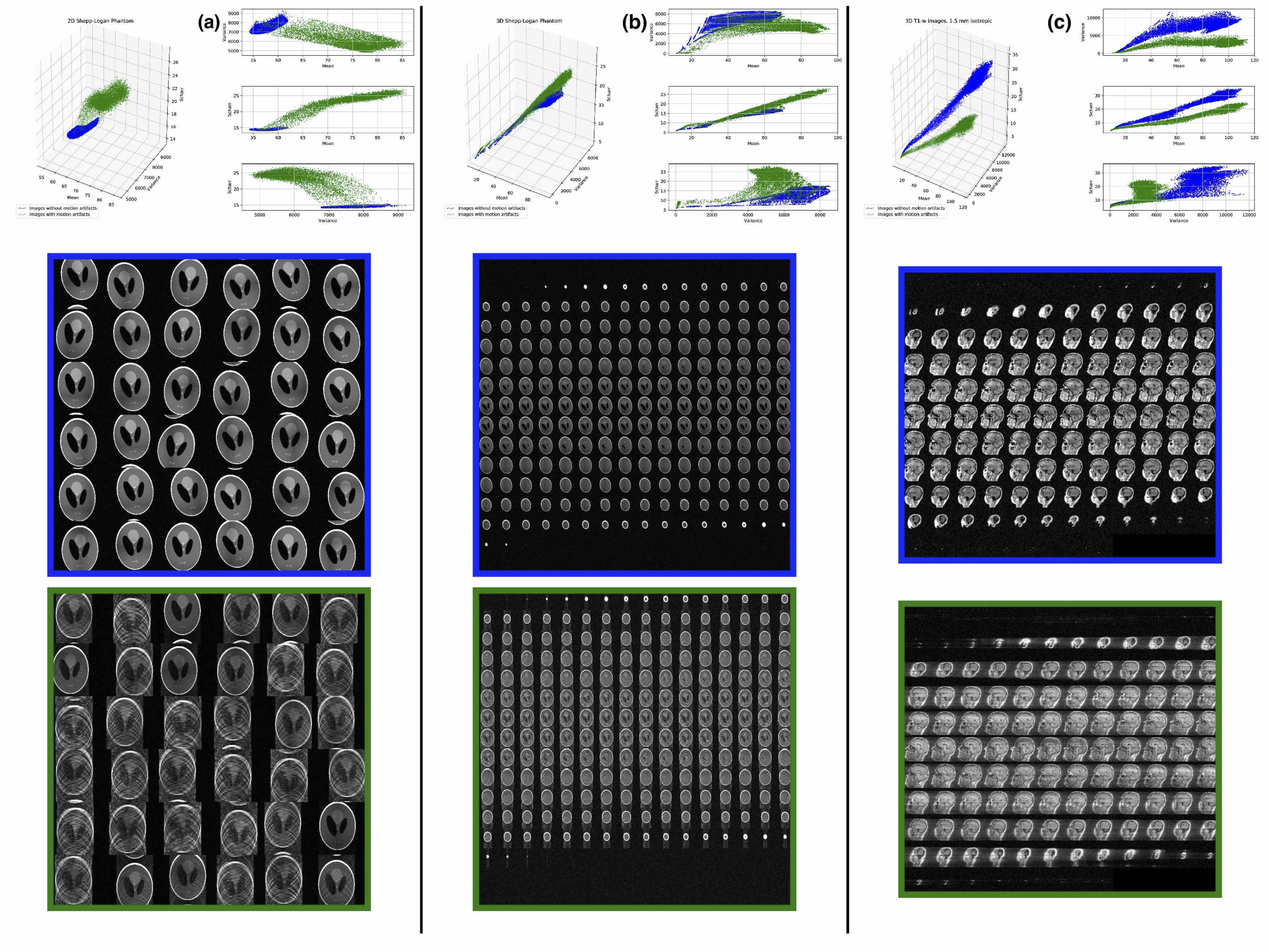
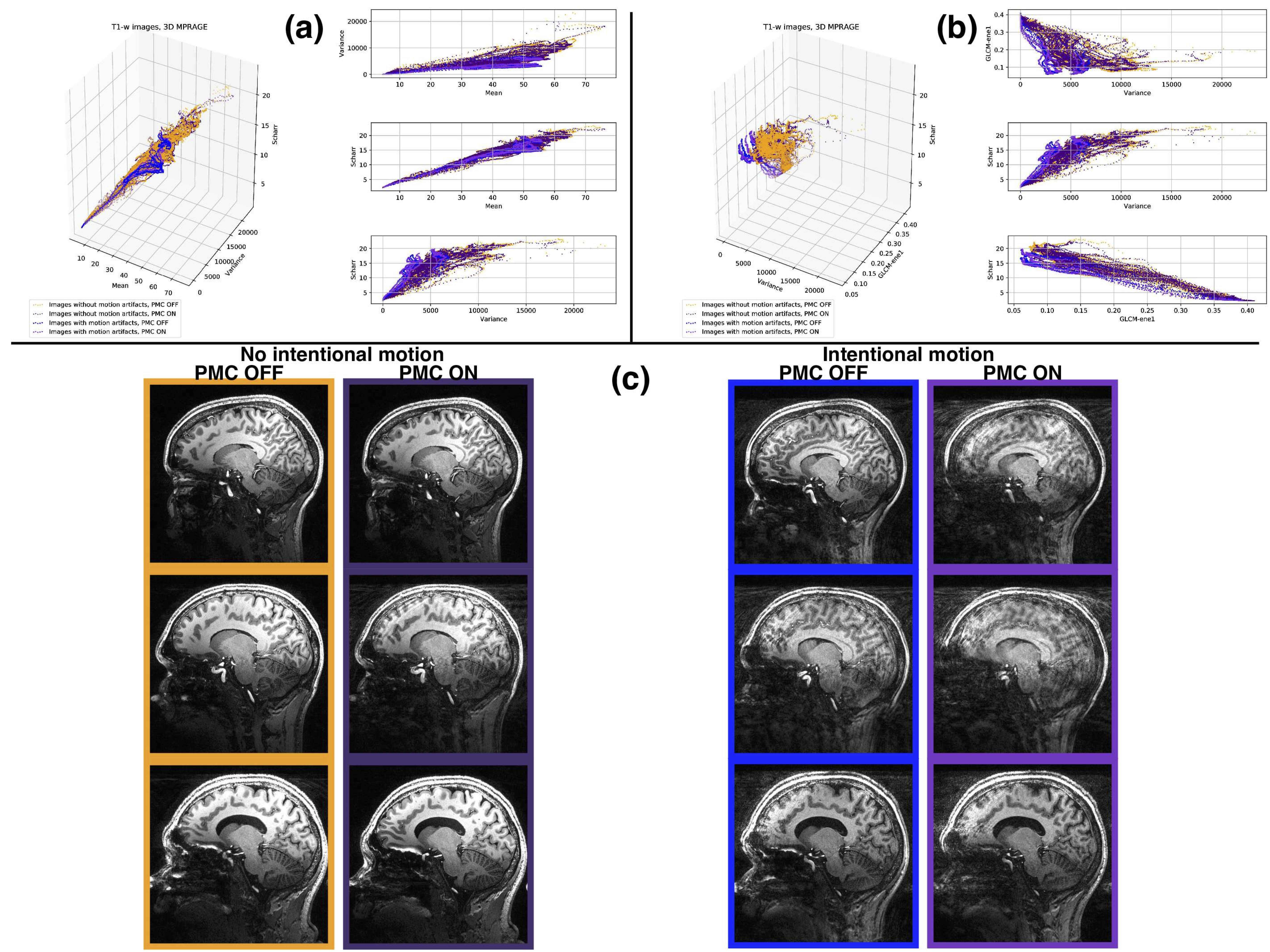
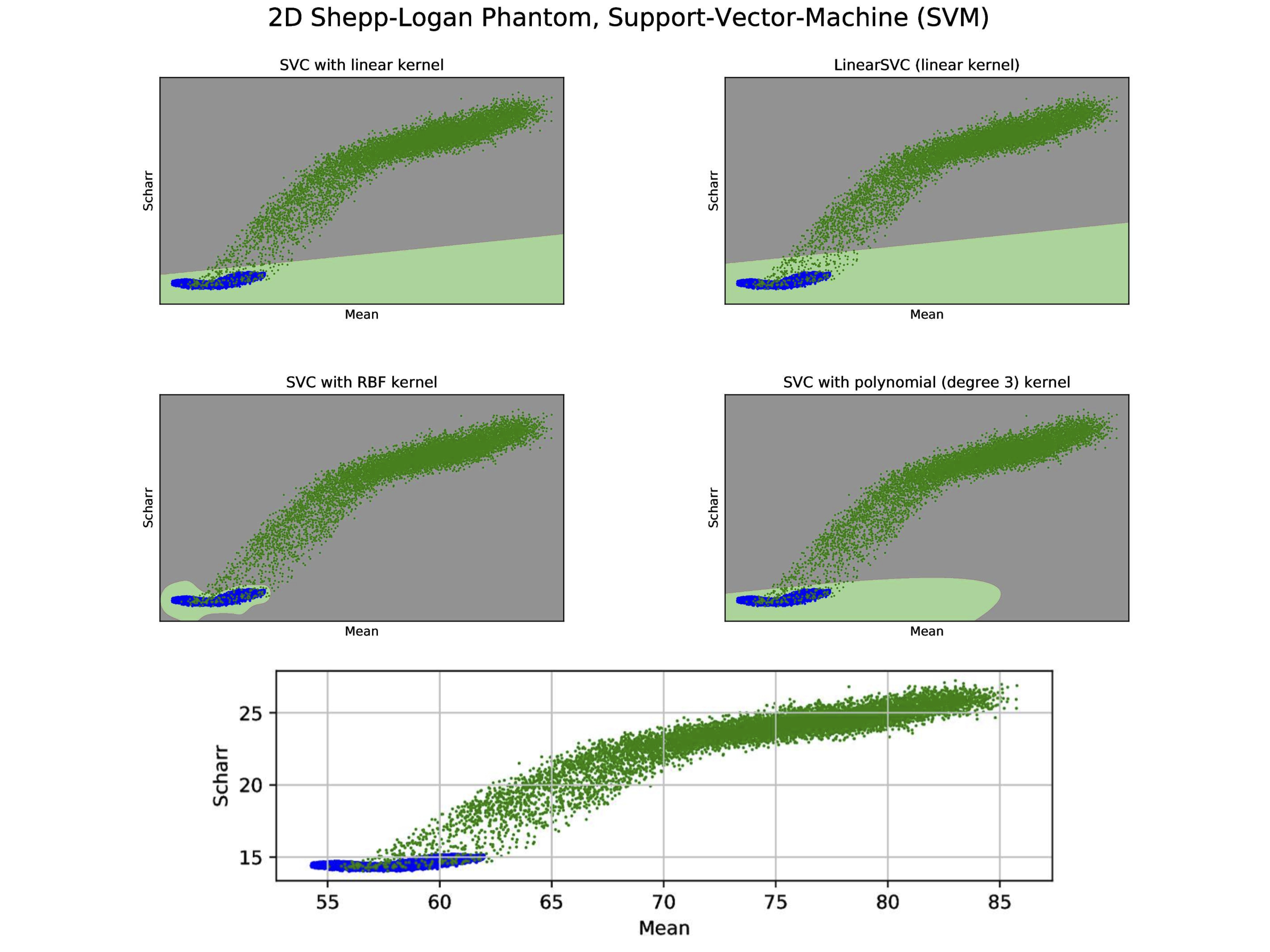
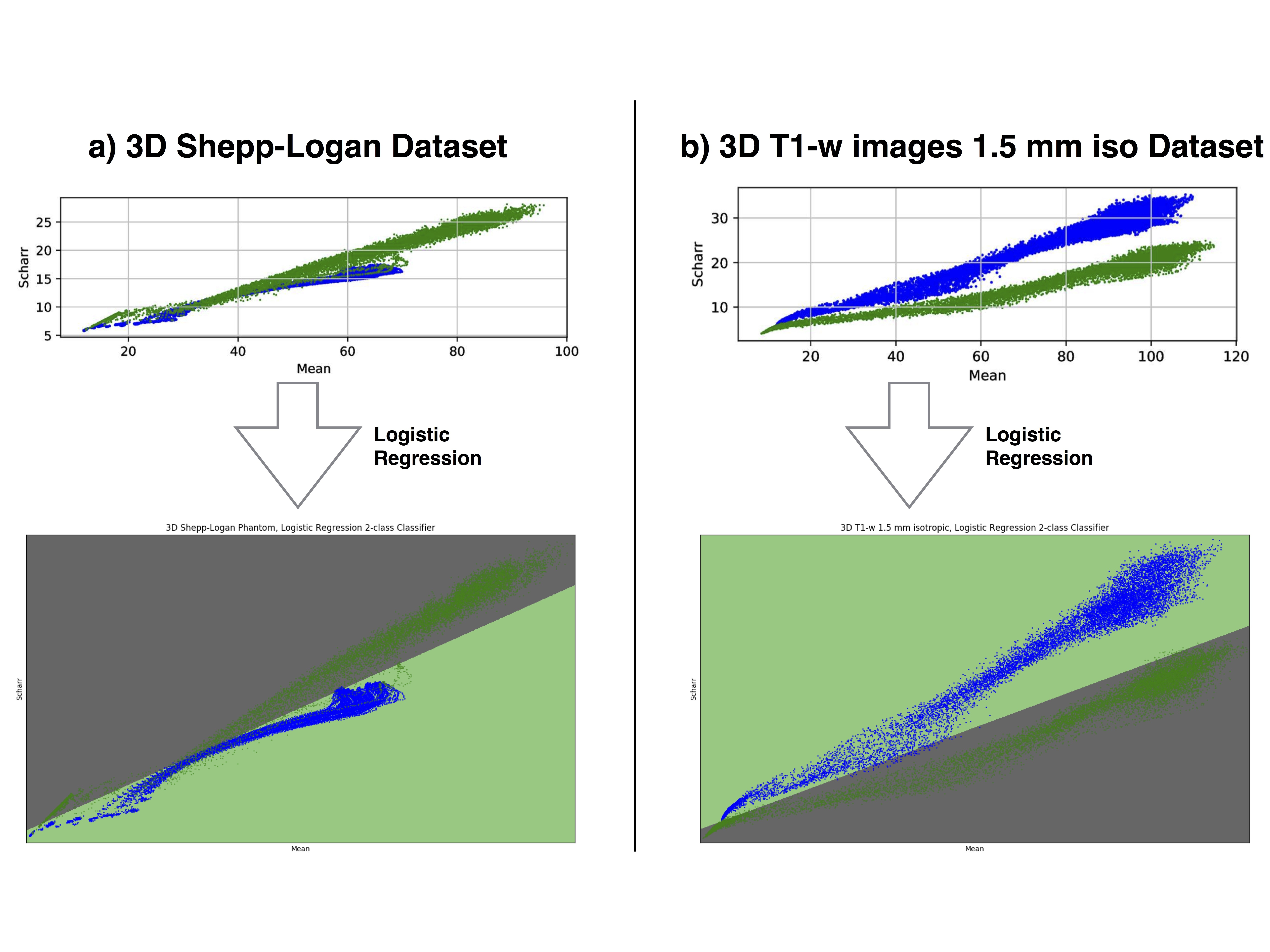
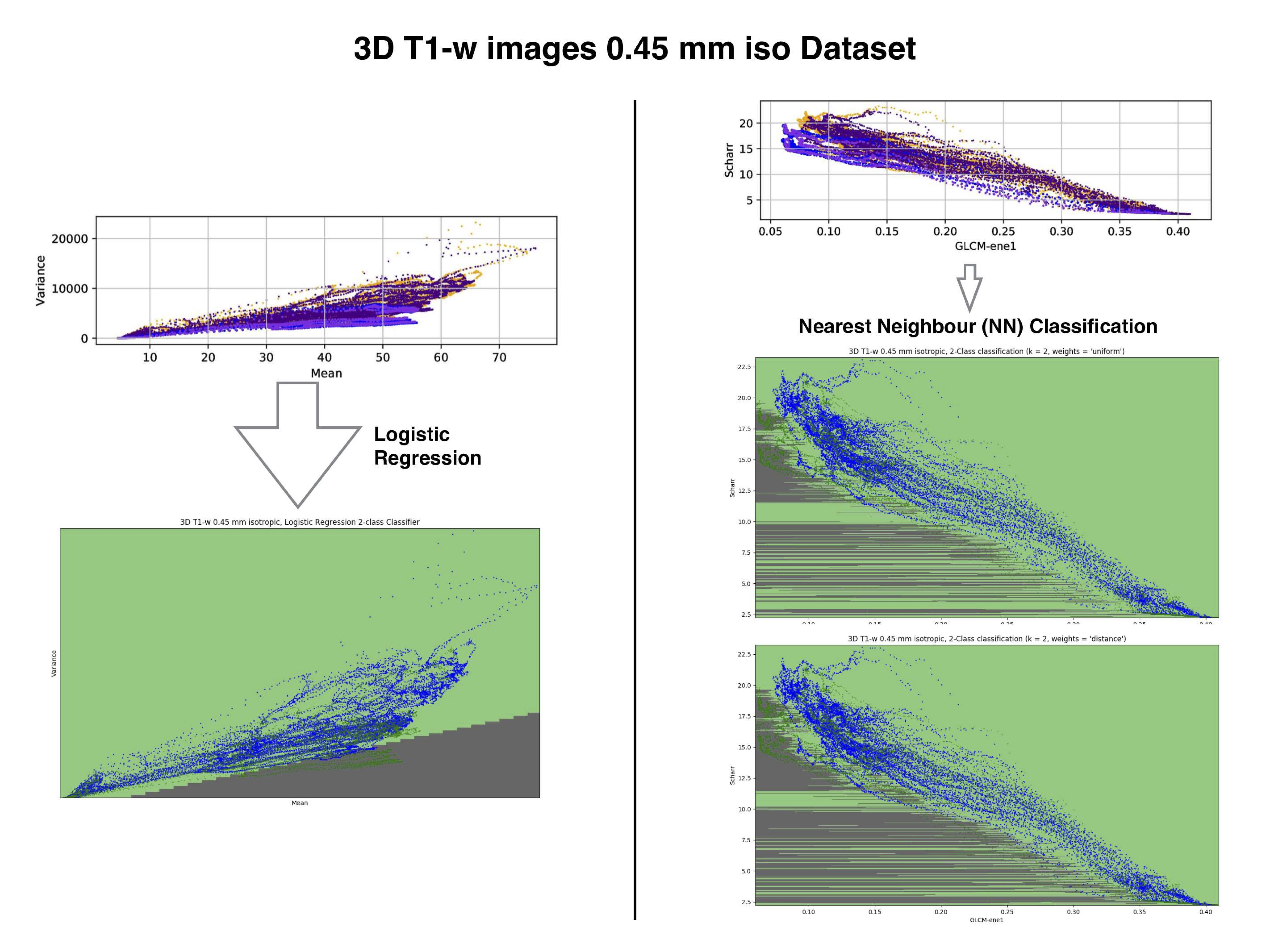
Fig. 5: Logistic Regression (left side) and Nearest Neighbors classification (right side) for the in-vivo 3D T1-w data set, 0.45 mm isotropic resolution.