4094
Using Machine Learning to accelerate fat-based head motion-navigators – a preliminary simulation study1CUBRIC, Cardiff University, Cardiff, United Kingdom
Synopsis
We hypothesise that machine learning approaches could be applied to speed up motion-correction navigators – potentially obviating the need for image reconstruction and co-registration. In this preliminary 2D simulation study we investigate the ability of a simple 5-layer convolutional neural network to predict motion-parameters based on difference images between two head poses. Our results indicate that the CNN is able to outperform linear regression over the range of parameters tested, supporting our aim to develop this concept in more detailed future work.
Introduction
We recently demonstrated that highly accelerated 3D-GRE acquisitions with a fat-excitation can be used effectively as high resolution head motion-navigators (3D-FatNavs) [1], with particular utility for imaging at ultra-high spatial resolution at 7T with extended scan-times [2]. To retain very high spatial fidelity we advocated a 2mm spatial resolution for the FatNavs, resulting in a 1152 ms navigator duration – even with 4x4 GRAPPA acceleration and ¾ partial Fourier undersampling in both PE directions. For sequences such as MP2RAGE or TSE which already have sufficient dead-time this navigator duration can be incorporated without affecting the overall scan-time – but for more universal applicability it is clear that a shorter navigator duration is desirable – ideally without sacrificing spatial resolution.
The current processing pipeline involves separately reconstructing each individual FatNav volume, then applying a rigid-body registration step to determine the 6 motion parameters to describe each head position over time. With a 32-ch receive coil, this corresponds to the acquisition of ~3 million datapoints with each 3D-FatNav in order to estimate only 6 parameters.
In this work we performed preliminary simulations to investigate the potential for applying a machine learning approach to allow high fidelity motion-tracking with a drastically shortened data acquisition. Our hypothesis is that even if the acquisition is so undersampled that no useful image can be reconstructed from it, the motion-information can still be encoded within the k-space data itself. A machine learning approach could then be used to learn the mapping between the acquired data and the rigid-body motion parameters.
Methods
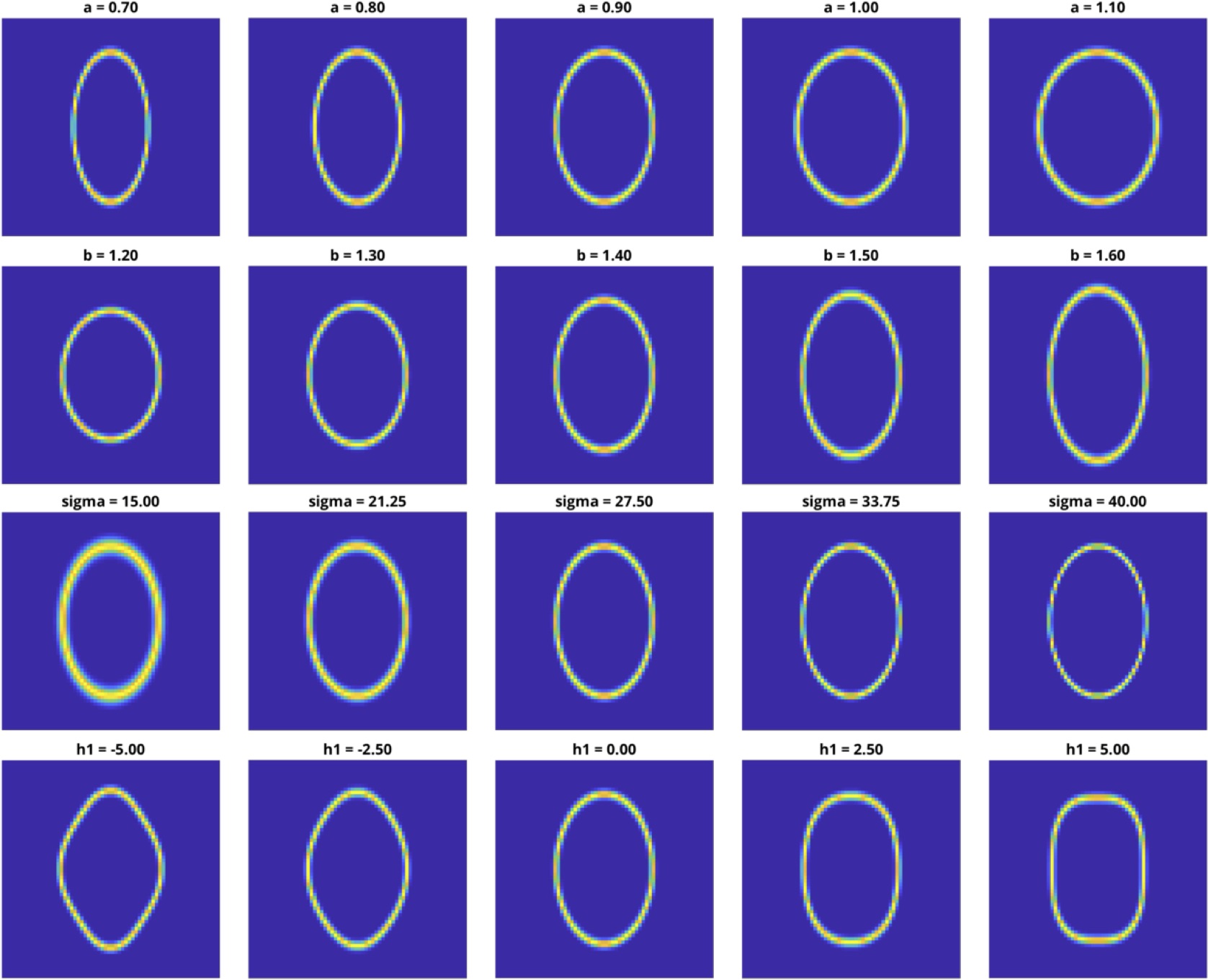
To create a simplified version of the problem for preliminary simulations, a 2D-ellipse was used to represent a sparse fat image of the head. The shape of the ellipse was parameterised with 4 variables (‘a’,’b’,’sigma’,’h1’) to create different forms representative of different human head shapes. These were not intended to be realistic modes of variation, but instead the aim was to introduce ‘natural variation’ to move beyond the simple case where the object is completely known prior to the experiment. The ranges of the parameters used are shown in Figure 1.
A pool of 20,000 ‘head pairs’ were then generated with random shape variables within the ranges described above on a 64x64 matrix size to use as the training data. The second image in the pair was generated by displacing the first by a random set of 3 rigid-body (2D) motion parameters within the ranges +-5 degrees and +-5 mm (the displacements were scaled so that a ‘millimetre’ could be defined relative to an approximate average head-size). The direct image subtraction between each pair was then Fourier transformed to create a k-space – and then subsampled to include just the central 30x30 k-space points. This would obviously not represent a drastic acquisition speed-up – but in this initial experiment we aimed first to establish whether a machine learning approach could outperform a direct linear regression, without needing to also consider the effect of the chosen k-space sub-sampling pattern. Gaussian noise was then added to each set of difference data after transforming back to the image domain at a scale of 1% of the maximum image intensity. All difference data were then represented by a 2D ‘difference matrix’ with dimensions 20,000 (no. of head pairs) x 900 (no. of data points per head pair).
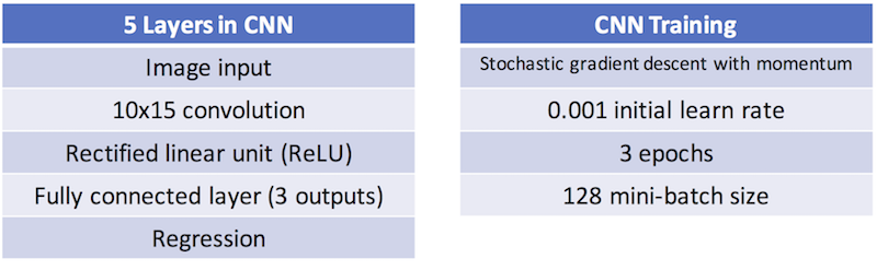
For linear regression, the pseudo-inverse of the difference matrix was multiplied by the matrix of motion parameters to create a matrix mapping between the two. To apply machine learning to the problem, the ‘Neural Network Toolbox’ in MATLAB R2017a (The MathWorks, Natick, MA) was used to create a convolutional neural network (CNN) with 5 layers (see Table 1). Training took ~3 minutes on a conventional laptop computer.
Both the linear regression method and the trained CNN were then used to estimate the motion parameters from a second set of 20,000 simulated head-pairs.
Results
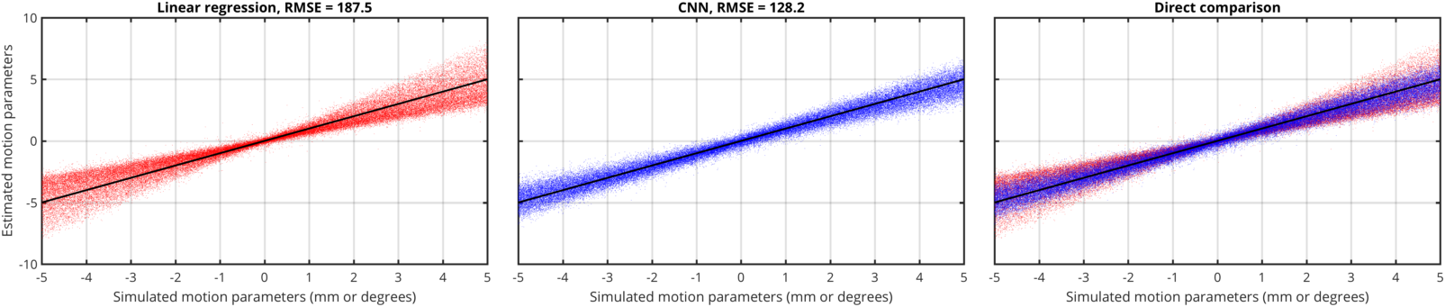
Figure 2 compares the ability of the linear regression and the trained CNN to predict the motion parameters from 20,000 new head-pairs. Linear regression shows a strong tendency to underestimate the motion parameters, whereas the CNN performs well throughout the simulated range. This is also reflected in the RMSE, which falls from 187.5 for the linear regression to 128.2 for the CNN.Conclusion
Clearly this preliminary 2D simulation is a very simplified version of the full 3D problem with multiple RF channels and natural variety in head shapes. Nonetheless, this study suggests that a machine learning approach may well be suitable for enabling faster motion-navigators, and will form the subject of future research.Acknowledgements
No acknowledgement found.References
[1] Gallichan, D., Marques, J.P., Gruetter, R., 2016. Retrospective correction of involuntary microscopic head movement using highly accelerated fat image navigators (3D FatNavs) at 7T. Magn. Reson. Med. 75, 1030–1039. doi:10.1002/mrm.25670
[2] Federau, C., Gallichan, D., 2016. Motion-Correction Enabled Ultra-High Resolution In-Vivo 7T-MRI of the Brain. PLOS One 11, e0154974. doi:10.1371/journal.pone.0154974
Figures