4091

A dynamic MR-signal model to capture 3D motion-fields at ultra-high frame-rate

Niek R.F. Huttinga^1,2, Cornelis A.T. van den Berg^1,2, Peter R. Luijten^1,2, and Alessandro Sbrizzi^1,2

¹Centre for image sciences, University Medical Centre Utrecht, Utrecht, Netherlands, ²Utrecht University, Utrecht, Netherlands

Synopsis

We present a framework that has the potential to capture non-rigid 3D motion at 50 Hz, hereby drastically accelerating state-of-the-art techniques. Our model directly and explicitly relates the motion-field to the k-space data and is independent of the spatial resolution, allowing for extremely high under-sampling. We illustrate proof-of-principle validations of our method through a simulation test and whole-brain 3D in-vivo measured data. Results show that the 3D motion-fields can be reconstructed from extremely under-sampled k-space data consisting of as little as 64 points, enabling 3D motion estimation at unprecedented frame-rates.

Introduction

Real-time estimation of three-dimensional human motion/deformation is crucial for applications such as MRI-guided radiotherapy and cardiac imaging. State-of-the-art dynamic MRI methods (e.g. navigators¹, cardiac gating² and low-rank compressed sensing³ aim at overcoming the inherently slow MR data encoding rate but are still far from achieving real-time, high-resolution, non-gated 3D acquisitions.

Here, we present a framework that has the potential to capture non-rigid 3D motion at 50 Hz, hereby drastically accelerating state-of-the-art techniques. Our model directly and explicitly relates the motion-field to the $$$k$$$-space data and is independent of the spatial resolution, allowing for extremely high under-sampling.

Preliminary numerical and in-vivo experimental tests show that reconstruction of an affine 3D motion-field is possible with as little as 64 $$$k$$$-space points.

Theory

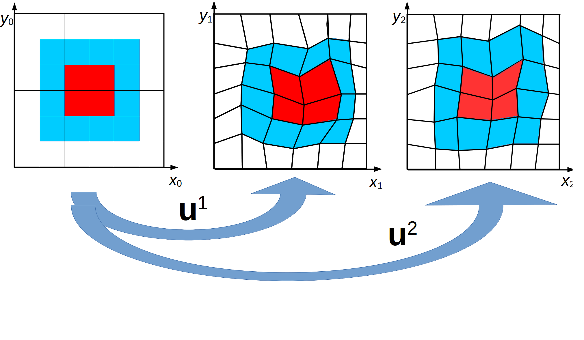
Our dynamic model directly relates the MR-signal of an object at time $$$t_{j+1}$$$ deformed by an unknown, possibly non-linear, motion-field $$$\boldsymbol{u}(\boldsymbol{r})$$$, to the reference image at time $$$t_j$$$ before deformation. The vector-field $$$\boldsymbol{u}$$$ thus induces a coordinate transformation between the two time points (Fig. 1):$$\boldsymbol{r}|_{t=t_j}\mapsto\boldsymbol{u}(\boldsymbol{r})|_{t=t_{j+1}}$$We assume that the magnetic spins are in the steady-state regime, thus\[m^{j+1}(\boldsymbol{r})=m^{j}(\boldsymbol{u}(\boldsymbol{r})).\] Here, the superscript indicates time and $$$m$$$ the (normalized) transverse magnetization. Additionally, we assume a spin-conservation relationship analogous to the mass-conservation:$$\rho^{j+1}(\boldsymbol{r})\text{d}\boldsymbol{r}=\rho^j(\boldsymbol{u}(\boldsymbol{r}))\text{d}\boldsymbol{u}(\boldsymbol{r})=\rho^j(\boldsymbol{u}(\boldsymbol{r}))\lvert J(\boldsymbol{u})\rvert\text{d}\boldsymbol{r}.$$Here, $$$\rho(\boldsymbol{r})$$$ denotes the spin density and $$$\lvert J(\boldsymbol{u})\rvert$$$ the determinant of the Jacobian of $$$\boldsymbol{u}$$$. Combining these assumptions and the change of variable formula for the multi-dimensional integral we arrive at the following formula for the signal at time $$$t_{j+1}$$$:$$s^{j+1}\left(\boldsymbol{k}\right)=\int_{\mathbb{R}^3}\rho^{j+1}(\boldsymbol{r})m^{j+1}(\boldsymbol{r})e^{-i 2\pi\boldsymbol{k}\cdot\boldsymbol{r}}\text{d}\boldsymbol{r}=\int_{\mathbb{R}^3}\rho^j(\boldsymbol{r})m^j(\boldsymbol{r})e^{-i 2\pi\boldsymbol{k}\cdot\boldsymbol{u}^{-1}(\boldsymbol{r})}\text{d}\boldsymbol{r}.$$In this work, we refer to $$$q^j(\boldsymbol{r}):=\rho^j(\boldsymbol{r})m^j(\boldsymbol{r})$$$ as the reference image and $$$s^{j+1}(\boldsymbol{k})$$$ as the snapshot data. Note that $$$\boldsymbol{u}(\boldsymbol{r})$$$ could represent non-linear/non-rigid transforms.

Methods

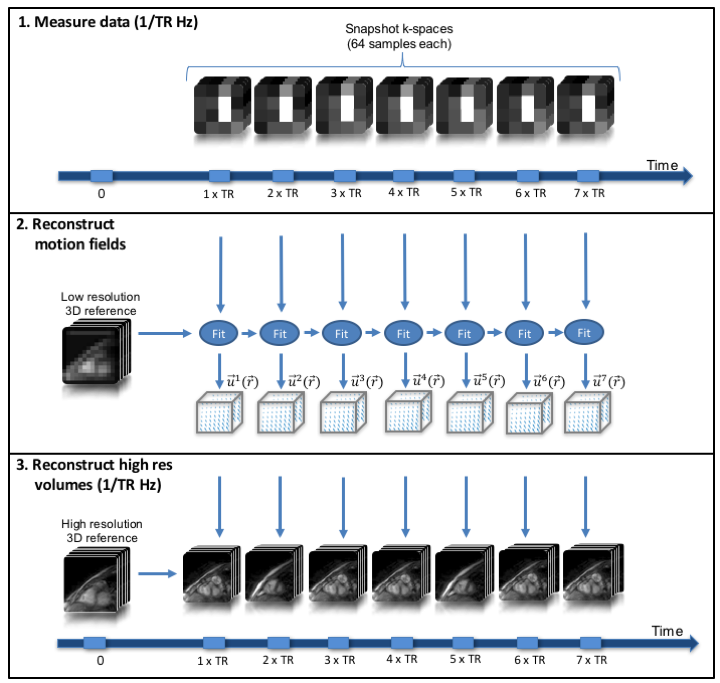
Given an MR-signal at time $$$t_{j+1}$$$ and a reference image at time $$$t_j$$$ we can reconstruct the deformation-field $$$\boldsymbol{u}(\boldsymbol{r})$$$ by numerically solving a non-linear inversion problem. See Fig. 2. We illustrate proof-of-principle validations of our method through a simulation test and whole-brain 3D in-vivo measured data.

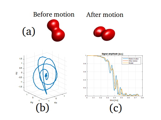
For the numerical test, we considered an affine transformation $$$\boldsymbol{u}(\boldsymbol{r})$$$, i.e. $$\boldsymbol{u}(\boldsymbol{r})=A\boldsymbol{r}+\boldsymbol{\tau},$$where $$$A\in\mathbb{R}^{3\times3}$$$ and $$$\boldsymbol{\tau}\in\mathbb{R}^3$$$. We employed a bSSFP sequence with a very short (sub-millisecond) 3D spiral readout trajectory (see Fig. 3). From the signal after motion (snapshot data) we reconstructed the affine transformation and compared the hereby deformed object with the ground-truth.

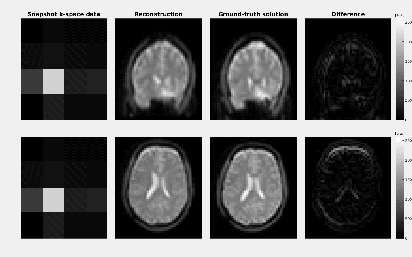
For the whole-brain 3D in-vivo test, we represented the motion-field by a non-rigid affine transformation. We acquired one reference image, and a total of seven snapshot $$$k$$$-spaces. The volunteer moved in between the scans. Data was acquired using a heavily under-sampled 3D steady-state SPGR sequence with Cartesian readout on a 1.5T MR system (Ingenia, Philips), TR/TE=8ms/3ms. Retrospectively down-sampling eventually resulted in a pre-motion reference image of size $$$34\times34\times34$$$ and $$$k$$$-space snapshots of size $$$4\times4\times4$$$ (i.e. 64 points acquired in $$$4\times4\times$$$TR=128ms). To obtain ground-truth images, we performed a 3D SPGR with a single-shot EPI readout (TR/TE=35ms/9ms) immediately after each snapshot scan.

Results

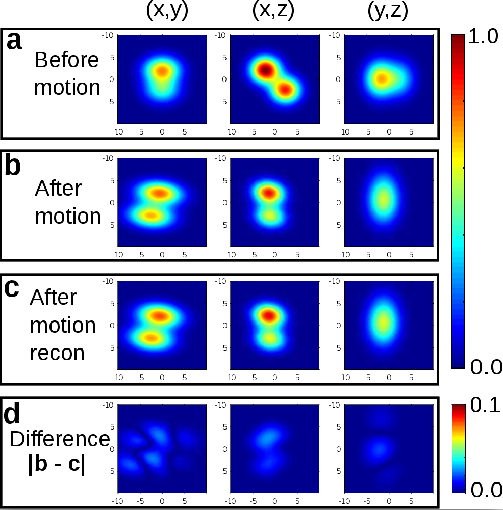
For the simulations, Fig. 3c shows that our model accurately predicts the true signal after motion. Fig. 4 shows the transformed object by applying the reconstructed motion-fields; a very high accuracy in the reconstruction is achieved.

Results of the in-vivo experiment are reported in Fig. 5 and show good agreement between our reconstruction and the ground-truth. We used a plain channel-wise sum of raw MR-signal data for our snapshots, lacking any form of channel sensitivity corrections. This possibly explains the difference in our reconstruction.

Discussion

We introduced a framework to reconstruct non-rigid 3D transformations from minimal MR-signal data. This study presented simulated and experimental proof-of-principle results, showing the potential of the method. In the future, we will employ fast single-shot spiral acquisitions and expect to achieve a high-resolution 3D acquisition protocol with 50 frames per second (TR=20ms).

While the head motion is described well by affine transformations, other organs (abdomen and/or heart) will require more local and non-rigid parameterizations for $$$\boldsymbol{u}$$$; splines and other compressed representations derived from existing 4D human models⁴ will be considered. Note that our proof-of-principle affine transformation reconstructions are obtained with only 64 points of Cartesian $$$k$$$-space. More sophisticated transformations may require different trajectories and/or more $$$k$$$-space points but should still fit in the targeted 50 Hz rate.

The highly under-sampled data leads to a reduced minimization problem, which could be solved in less than a second with our initial Matlab implementation. Real-time reconstruction should be obtained by making use of CUDA/GPU implementations.

Conclusion

We derived a new MR-signal model which directly and explicitly relates the measured data to the motion/deformation-field. Simulations and experimental proof-of-principles show that these fields can be reconstructed from extremely under-sampled $$$k$$$-space data, enabling 3D motion estimation at unprecedented frame-rates.

Acknowledgements

This research is funded by the Netherlands Organisation for Scientific Research, domain Applied and Engineering Sciences, Grant number: 15115.

References

Welch, E. B., Manduca, A., Grimm, R. C., Ward, H. A., and Jack Jr, C. R. Spherical navigator echoes for full 3D rigid body motion measurement in MRI. Magnetic Resonance in Medicine 47 , 1 (2002), 32–41.
Uribe, S., Muthurangu, V., Boubertakh, R., Schaeffter, T., Razavi, R., Hill, D. L., and Hansen, M. S. Whole-heart cine MRI using real-time respiratory self-gating. Magnetic Resonance in Medicine 57 , 3 (2007), 606–613.
Otazo, R., Candès, E., and Sodickson, D. K. Low-rank plus sparse matrix decomposition for accelerated dynamic MRI with separation of background and dynamic components. Magnetic Resonance in Medicine 73 , 3 (2015), 1125–1136.
Segars, W., Bond, J., Frush, J., Hon, S., Eckersley, C., Williams, C. H., Feng, J., Tward, D. J., Ratnanather, J., Miller, M., et al. Population of anatomically variable 4D xCAT adult phantoms for imaging research and optimization. Medical physics 40 , 4 (2013).

Figures

Figure 1: Organ motion/deformation modeled as a change of variables transformation. The reference grid is transformed by the function, $$$\boldsymbol{u}^j$$$, into a new coordinate system.

Figure 2: Schematic overview of the proposed method. First, we acquire very low-resolution snapshot data from a moving object (step 1). Using a fast single-shot readout (e.g. TR=20ms), this implies a high-resolution 3D acquisition at a rate of 1/TR=50 Hz. Next, we reconstruct the desired motion-fields from the snapshots and a low-resolution reference image (step 2). Noise and small motion-artifacts will be reduced in these images, making the proposed method more robust. Optionally, we can reconstruct high-resolution 3D images by applying the reconstructed motion-fields to a high-resolution reference (step 3).

Figure 3: The results of the numerical validation of the model. (a): Analytical object before (left) and after (right) deformation. (b): The implemented very short (sub-millisecond) single-shot 3D spiral $$$k$$$-space trajectory used for the snapshot acquisitions. (c): Plot of the amplitude of the true signal before motion (blue), true signal after motion (red) and signal from our model (orange) versus acquisition time. Note that the signal after motion is accurately described by the model (red and orange lines coincide).

Figure 4: Results from 3D motion reconstruction. Axis are in [cm]. Image values are [a.u]. (a): Slices of the object before motion in transversal (left), axial (middle) and sagittal (right) planes. (b): Slices of the object after motion. (c): Slices of the object after motion reconstructed by our model. (d): Slices of the absolute difference between ground-truth images in (b) and reconstructed images in (c).

Figure 5 (animated): Results of the reconstruction on whole-brain in-vivo data. From left-to-right we show the highly under-sampled input $$$k$$$-space data, the reconstruction of our model, the ground-truth solution and the absolute difference between the two images. The top-row images show slices in axial direction, and the bottom-row images show slices in transversal direction. The animation shows the reconstructed images over time.

Proc. Intl. Soc. Mag. Reson. Med. 26 (2018)

4091