4086
Evaluating Motion Artifact Correction of the Linearized Geometric Solution in bSSFP MRI1Radiology, University of Washington, Seattle, WA, United States, 2Radiology, University of British Columbia, Vancouver, BC, Canada, 3Physics, University of British Columbia, Vancouver, BC, Canada
Synopsis
The linearized geometric solution (LGS) is known for demodulating balanced steady state free precession (bSSFP) MRI signal of its dependence on magnetic field inhomogeneity, but has also recently shown signs of mitigating motion artifact. Here the extent of motion artifact correction by the LGS is explored via simulations of variable motion schedules, image noise, and T1/T2 ratio. It corrects motion artifact to a greater extent than a complex image averaging solution, except in scenarios of low signal-to-noise ratio (SNR). This study motivates clinical applications of bSSFP in imaging fluid structures that normally suffer from motion and/or field inhomogeneity artifacts.
Introduction
Recent indications that the Linearized Geometric Solution (LGS) mitigates motion artifacts1 in balanced steady state free precession (bSSFP) MRI are intriguing, given that the LGS already eliminates magnetic field imhomogeneity-induced signal modulation/banding2. The ubiquity and diagnostic detriment of MRI motion artifacts inspires an evaluation of the LGS’ capacity for motion artifact correction, to better ascertain its utility for future clinical use.Methods
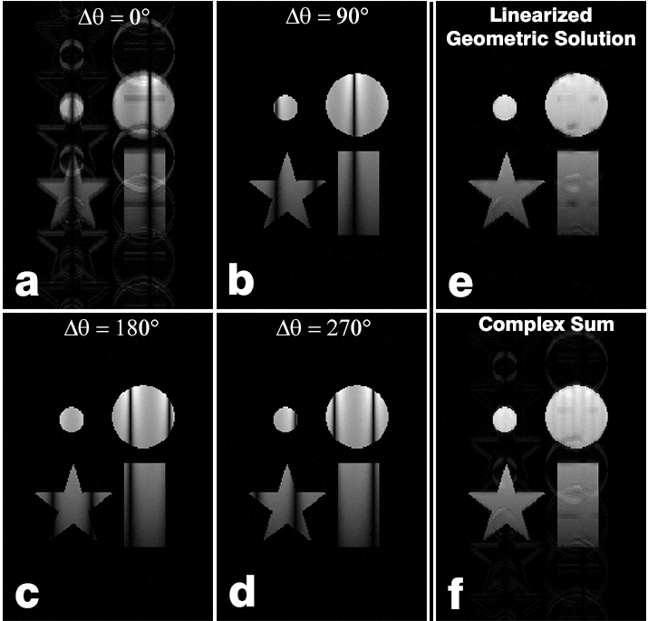
Four $$$\Delta\theta$$$ = 0°, 90°, 180°, and 270° respectively radiofrequency (RF) phase-cycled bSSFP datasets were simulated with flip angle = 70°, repetition time = 4.2ms, and spatially-varying T1 relaxation from 200 to 3000 ms, T2 relaxation from 40 to 3000 ms, and off-resonant accumulated phase $$$\theta$$$ from -4$$$\pi$$$ to +4$$$\pi$$$. Magnitude data were multiplied by a binary mask of basic shapes to introduce structure. Motion was simulated as follows3: the $$$\Delta\theta$$$ = 0° dataset’s signal region was incrementally translated in one dimension to oscillate at a specific frequency and amplitude. A 2D Fourier Transform (FT) was applied to each motion frame to yield a stack of k-space frames that together formed a 3D k-t space. This 3D data was obliquely sampled by assembling spatially-sequential lines (parallel to the motion direction for “PE motion”, perpendicular to the motion direction for “FE motion”) from temporally-sequential k-space frames to form a motion-corrupted k-space. An inverse 2DFT was applied to yield the motion-corrupted image, such as shown in Fig. 1a for motion amplitude: 3 pixels and frequency: 40 cycles/dataset. Zero-mean gaussian noise was added to this image and the uncorrupted $$$\Delta\theta$$$ = 90°, 180°, and 270° phase-cycled bSSFP images (Fig. 1b-d). The LGS (Fig. 1e) and a complex sum4 (CS, Fig. 1f) were computed pixel-by-pixel on the four phase-cycled images (one corrupted by motion) as previously described2.
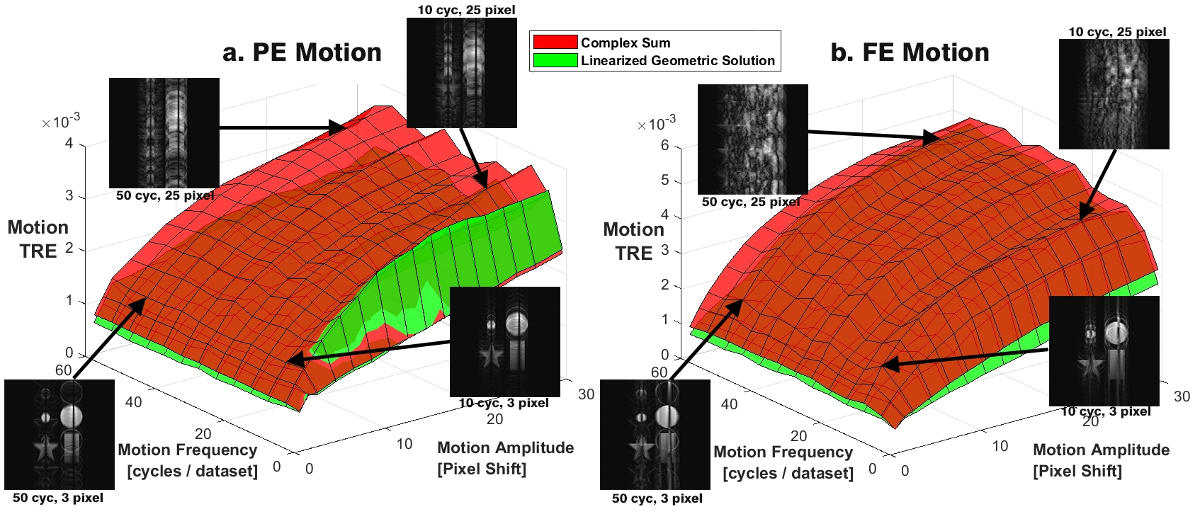
Figure 2 and 3 plot the total relative error (TRE) $$\frac{\sqrt{\sum{(|I_{LGS\,or\, CS}|-|I_{gold}|})^2}}{\sum|I_{gold}|}$$ of the LGS ($$$I_{LGS}$$$ in green) and CS ($$$I_{CS}$$$ in red). This error is calculated relative to ($$$I_{gold}$$$), which in this case is the LGS and CS of a phase-cycled dataset without motion corruption. This permits error quantification of only the motion artifact, and ignores error associated with magnetic field inhomogeneity artifact.
Figure 2 computes the TRE for a. PE motion and b. FE motion at variable motion frequency and amplitude in order to generate 3D surface error plots for the LGS and CS. Both PE and FE motion plots are annotated with four $$$\Delta\theta$$$ = 0° images corrupted by motion of varied parameters to give a sample of contributing data.
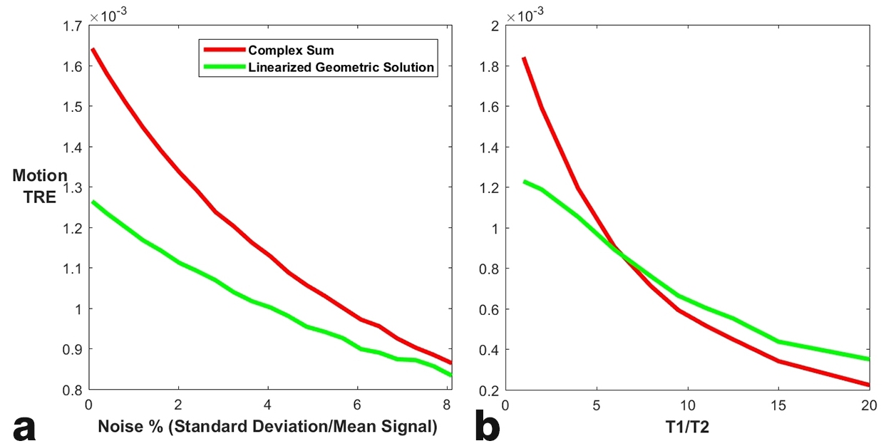
Figure 3a depicts LGS and CS TRE values calculated from bSSFP data similar to Fig. 1a-d, but at variable noise values. Figure 3b depicts TRE as a function of T1/T2 ratio: several bSSFP datasets similar to Fig. 1a-d are generated with variable tissue-emulating T1/T2 ratios, where T1 and T2 are spatially constant within each dataset. The LGS and CS are computed for each dataset, and TRE subsequently calculated.
Results
Figure 1 demonstrates that the LGS has visually better image quality than the CS, with less artifacts from both motion and banding. This is confirmed by Fig. 2, with the exception of some scenarios with low-frequency, mid-to-high-amplitude PE motion. Figure 3 shows that the LGS provides better motion correction than the basic averaging of the CS for the higher signal-to-noise (SNR) images that occur at lower T1/T2 ratios or image noise. However, the CS performs similarly or better for images with lower SNR due to higher T1/T2 or image noise.Discussion
This study confirms that beyond correction of magnetic field inhomogeneity artifacts, the LGS has the propensity for motion artifact mitigation in bSSFP imaging. Image ghosts seen in noise regions are eradicated, and LGS motion artifact correction is more extensive than the standard CS averaging of multiple phase-cycled datasets. However, motion artifacts in signal regions are still present, and can even exceed those in CS images at low SNR levels that occur when T1/T2 > 6. High T1/T2 ratio tissues such as liver, muscle, and brain matter yield low SNR in bSSFP imaging, where basic complex image averaging offers good results. However, bSSFP imaging is clinically employed for visualization of low T1/T2 tissue such as blood and cerebrospinal fluid, where the LGS’ correction of motion (and magnetic field inhomogeneity) artifacts tops the CS.Conclusion
The LGS reconstruction bolsters the clinical viability of bSSFP imaging by mitigating motion artifacts in addition to its previously validated ability to correct signal modulation/banding.Acknowledgements
No acknowledgement found.References
1. Hoff MN, Wilson GJ, Xiang Q-S, Andre JB. Artifact Correction in Temporal Bone Imaging with GS-bSSFP. In: Proc. ISMRM, Milan, Italy, 2014. p. 1627.
2. Xiang Q-S, Hoff MN. Banding Artifact Removal for bSSFP Imaging with an Elliptical Signal Model. Magn Reson Med, 2014; 71(3):927-933.
3. Xiang Q-S, Henkelman, RM. K-space description for MR imaging of dynamic objects. Magn Reson Med, 1993; 29(3):422-428.
4. Ernst RR. Fourier Transform NMR Spectroscopy Employing a Phase Modulated RF Carrier. US Patent 3,968,424. July 6, 1976.
Figures