Introduction

Magnetic Resonance Fingerprinting (MRF) uses a highly undersampled time-point series acquisition to simultaneously estimate T₁, T₂ and other quantitative parameters¹. Although MRF benefits from some motion resistance¹, persistent motion throughout the acquisition can create artefacts in the resulting parametric maps^2,3,4. Self-contained motion correction methods are desirable in MRF, to avoid altering the magnetization state. Self-navigation methods derive motion models from k-space data itself, but may fail in dynamic contrast acquisitions such as MRF. Here we investigate a method to obtain a 1D model of the motion via zero-dimensional (central k-space point) self-navigation in MRF using Independent Component Analysis (ICA). The estimated 1D motion model, however, is only accurate up to a scaling factor and may have residual errors. Therefore an autofocus⁵ algorithm is employed to further improve motion estimation and correct the k-space data.

Methods

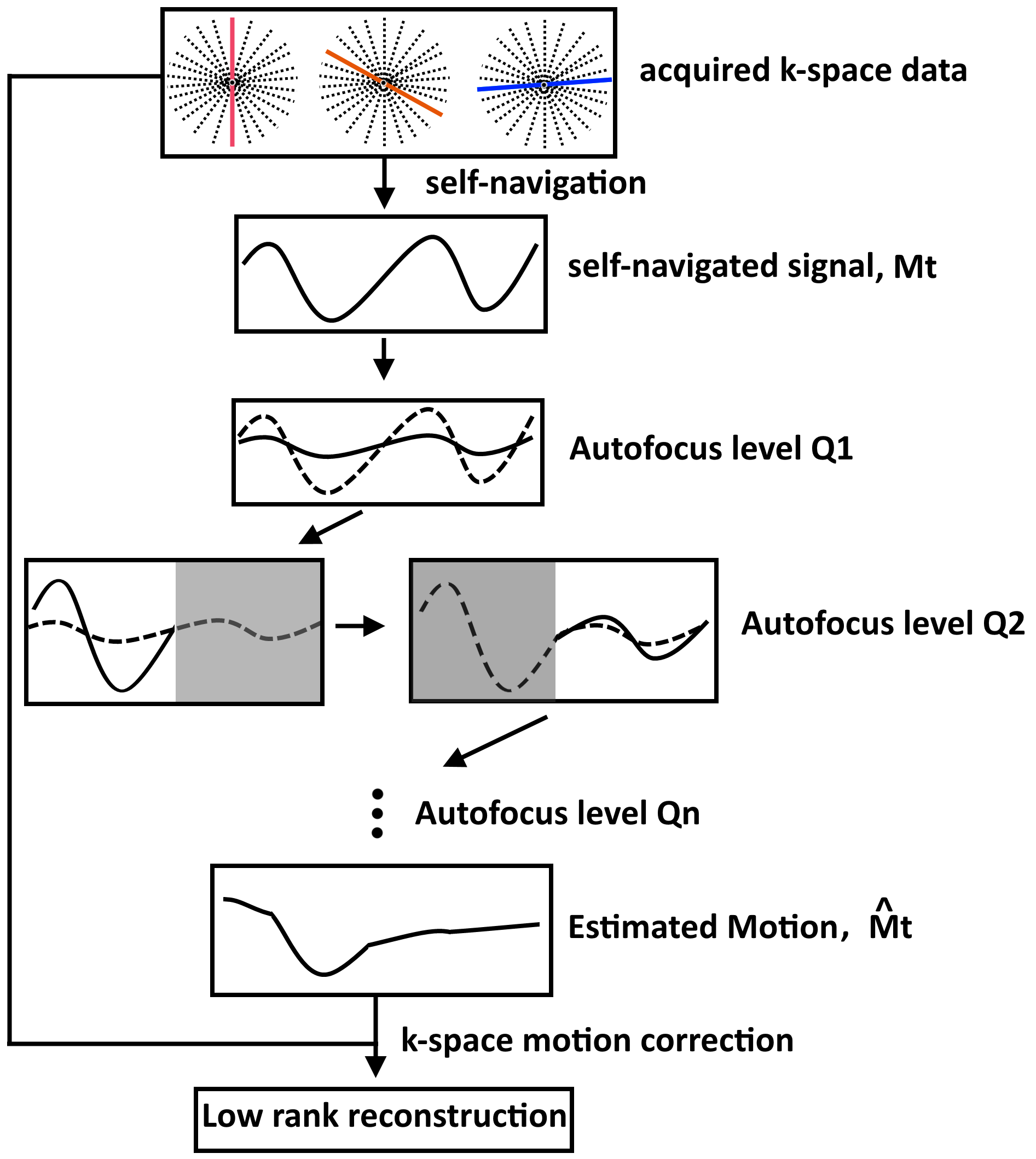
Self-navigation in dynamic contrast acquisitions is challenging since variations in k-space data can result from both motion and varying magnetization states. The proposed self-Navigated AUtofocus (NAU) approach consists of three steps: 1) a zero-dimensional self-navigation step to obtain an intermediate 1D motion estimation M_t, 2) an autofocus algorithm to obtain a further refined motion estimation $$$\bf{\hat{M}_t}$$$ , and 3) a low-rank inversion⁶ motion corrected reconstruction. Self-navigation is achieved by normalizing the k-space centre at each time-point k_t(0) by the energy $$$ \bf{E_t = \sum_r X_t(r)} $$$ of each time point image X_t(r), where X_t(r) is a motion-corrupted low-rank reconstruction of the time point series (pixel r, time-point t). Filtering and ICA are applied to the normalized self-navigated signal to obtain M_t. Although we expect M_t to capture 1D motion, it may be incorrectly scaled and may have errors resulting from static tissues and residual contrast variation. We further refine M_t iteratively in the second step of NAU using a hierarchical autofocus algorithm with a local gradient entropy metric $$$\bf{H(X) = \sum_b \{ {-\sum_r{X'(r)_b log[X'(r)_b]}}} \}$$$, where X’(r)b is the spatial gradient around block b of image X. To reduce the number of unknowns, we look for $$$ min_{\alpha , \beta} H(\hat{X}_t) $$$, where $$$\bf{\hat{X}_t}$$$ is the motion-corrected time-point series using the 1D motion model $$$\bf{\hat{M}_t} = \alpha \bf{M_t} + \beta$$$. A diagram of the NAU framework is depicted in Figure 1. The final $$$\bf{\hat{M}_t}$$$ is used to correct the acquired k-space data, followed by a final (motion corrected) low rank reconstruction.

Experiments

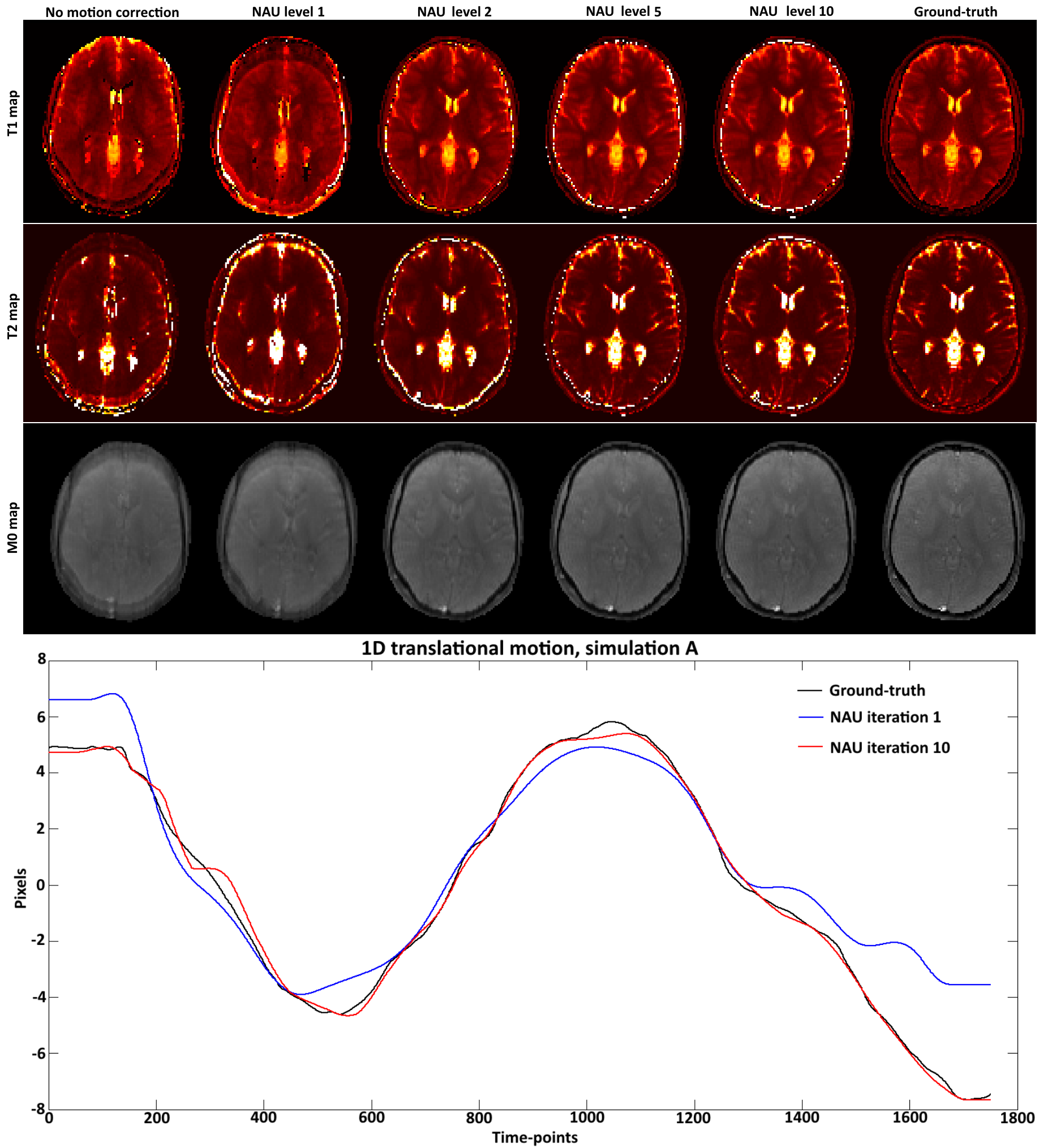
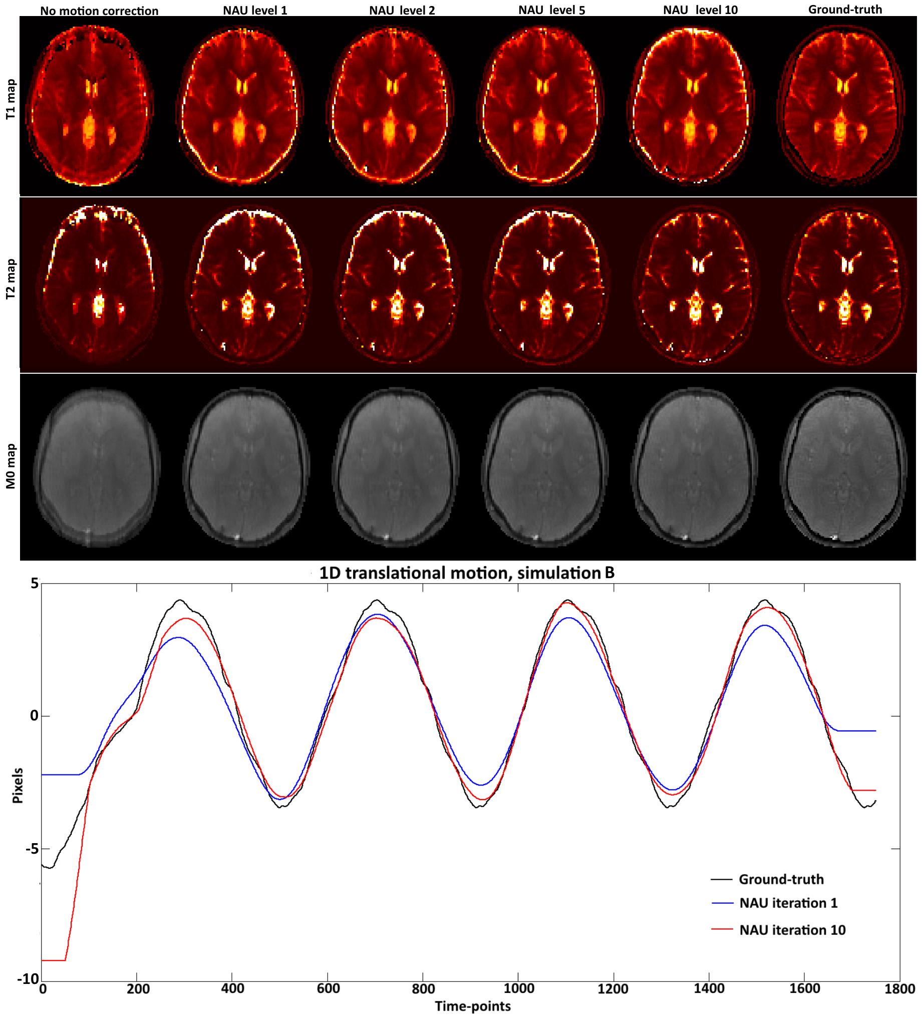
A digital phantom modelled after a brain image with realistic T₁ and T₂ values was used to simulate an MRF acquisition with a sequence similar to⁷ under periodic 1D translational motion. Two different simulated motions (A and B) were tested. The simulated acquisition was based on: fixed TE/TR = 1.2/4.3 ms, Nt =1750 time-points, golden radial trajectory with a single spoke per time-point. The optimization for $$$\alpha$$$ and $$$\beta$$$ was performed via exhaustive search at each hierarchical level l = 1,…,10. Each hierarchical level divide the motion model in $$$Q_l$$$ = [1 2 3 5 7 11 13 17 19 23] segments in time. Thus at each level the autofocus algorithm modified $$$N_t / Q_l$$$ time-points at a time. Localized gradient entropy was measured on a block size b = 23 pixels. The low rank approximation used a rank r = 15 and Conjugate Gradient with 15 iterations.

Results

T₁, T₂, M₀ maps and estimated motion from different hierarchical levels of the proposed NAU for simulated motions A and B are shown in Figures 2 and 3, respectively. A gradual improvement of sharpness can be observed as the algorithm resolves motion at smaller temporal resolutions in later iterations. The simulated motion plots show the result of the initial global autofocus estimated motion (hierarchical level 1) as well as the last (hierarchical level 10), which is closer to the ground-truth.

Conclusion

The proposed NAU method introduces a self-navigated autofocus solution for MRF motion correction. The proposed approach has the potential for motion estimation at high temporal resolution. Proof of concept was demonstrated in simulations achieving similar quality to the ground-truth T₁/T₂ maps. Future work will investigate feasibility in-vivo and more complex motion models⁸ using more efficient optimizations⁹.

Acknowledgements

ACKNOWLEGDMENTS: This work was supported by EPSRC EP/P001009/1 and FONDECYT 1161055.