4060
Estimation of RF-induced temperature rise for helix and straight leads based on the lead electromagnetic model: a case study1Max Planck Institute for Human Cognitive and Brain Sciences, Leipzig, Germany, 2U.S. FDA, CDRH, Office of Science and Engineering Laboratories, Division of Biomedical Physics, Silver Spring, MD, United States
Synopsis
This case study investigated RF-induced heating of straight and helix leads at 127.7 MHz obtained with the lead electromagnetic model (LEM) and direct 3D electromagnetic and thermal co-simulations. A large set of incident electric fields was generated in a phantom by an array of four antennas with varying spatial positions and sources. LEM was a suitable approach for predicting temperature in close proximity to the end face of lead tip. However the variance of the fitted values and observed values was rather high for temperature at other locations around the lead tip.
Introduction:
One approach to evaluate RF-induced heating near an active implantable medical device (AIMD) lead is the lead electromagnetic model (LEM) prescribed in Clause#8 of ISO/TS_10974_Ed2 [1]. Using the transfer function (S(l)) [2] the LEM relates the incident tangential electric field (Etan) along lead trajectory to the RF power deposition (P) and temperature rise at a given point in space (ΔTp) due to presence of the lead. In the LEM
$$P = A\cdot\left[\int_{0}^{L} S(l)\cdot E_{tan}\cdot dl \right]^{2}$$
$$\triangle T_{p} = A_{T_{p}}\cdot\left[\int_{0}^{L} S(l)\cdot E_{tan}\cdot dl \right]^{2}$$
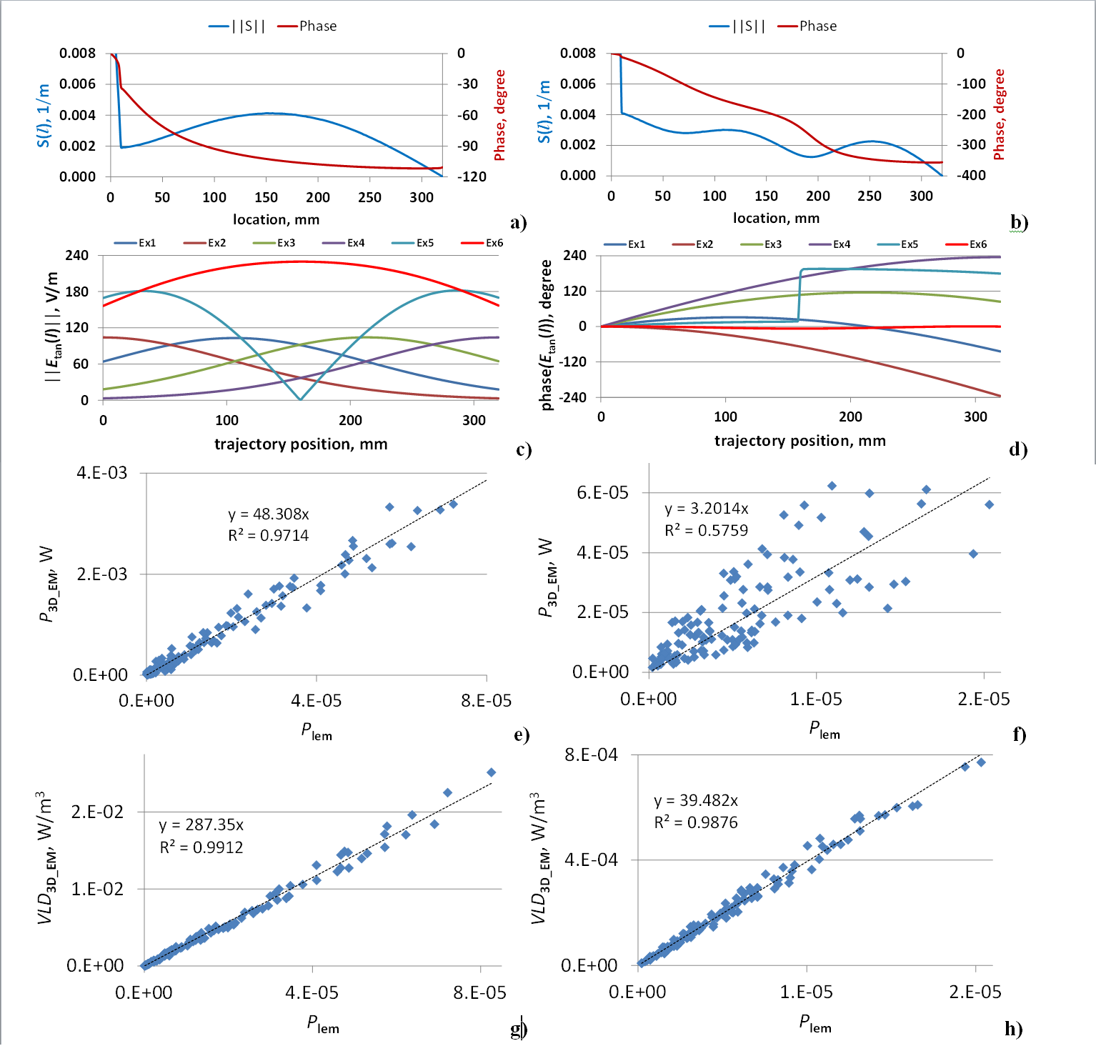
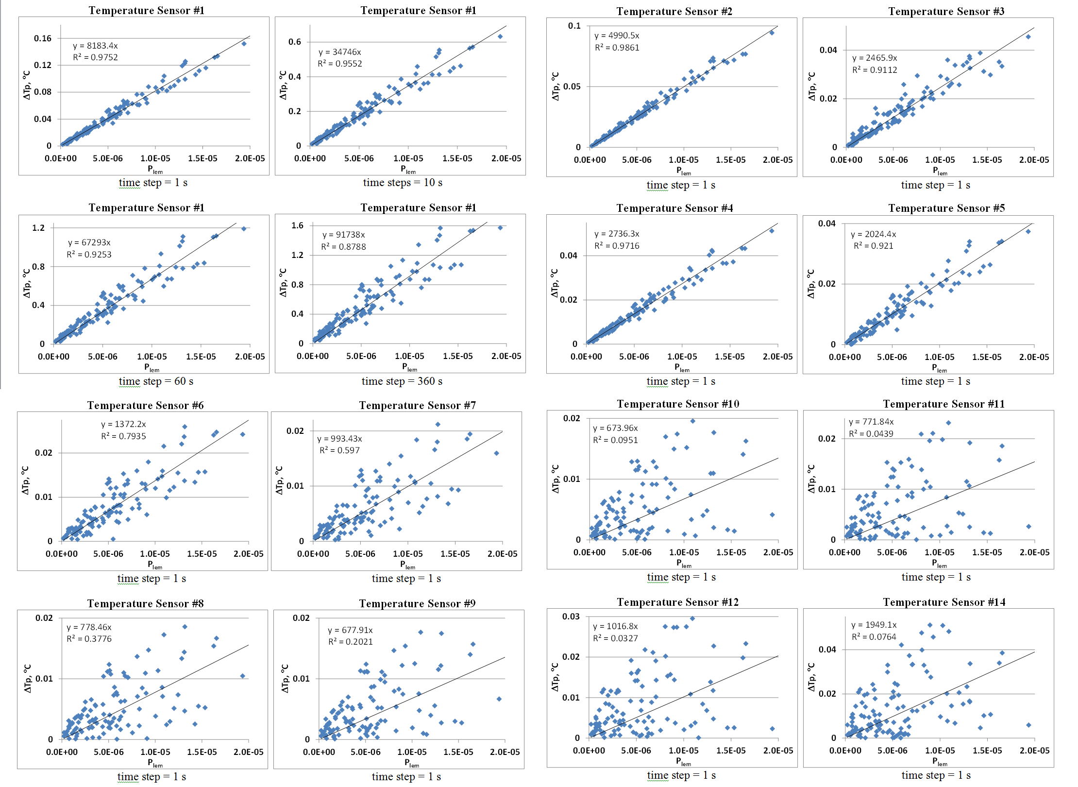
where: A and ATp are the calibration factors of the LEM for P and ΔTp, respectively, and L is the lead length. Both calibration factors can be assessed using a linear regression analysis of P and ΔTp versus $$$P_{lem} = \left[\int_{0}^{L} S(l)\cdot E_{tan}\cdot dl \right]^{2}$$$ obtained for a set of diverse non-uniform Etan(l). The associated regression coefficients R2A and R2ATp are the quotient of the variances of the fitted values and the observed values of the dependent variable. Etan(l) disturbance depends on the proximity between the implant segments and the construction of the implant. The smallest disturbance of Etan(l) occurs for the straight lead trajectory allowed the most reliable estimation of A and ATp.
Methods:
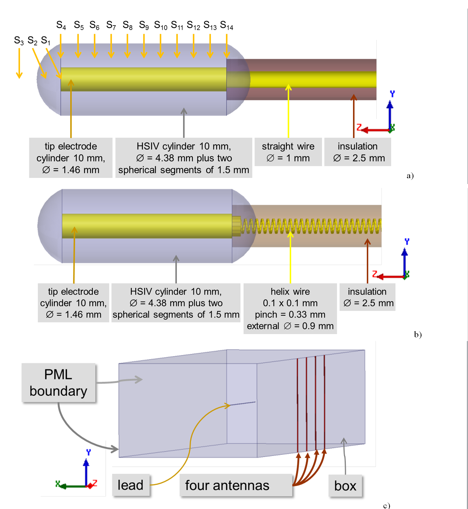
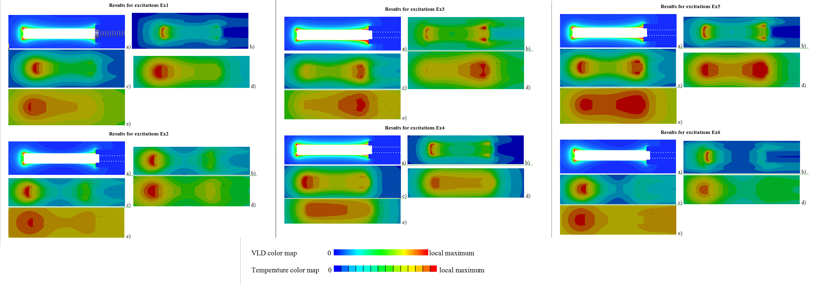
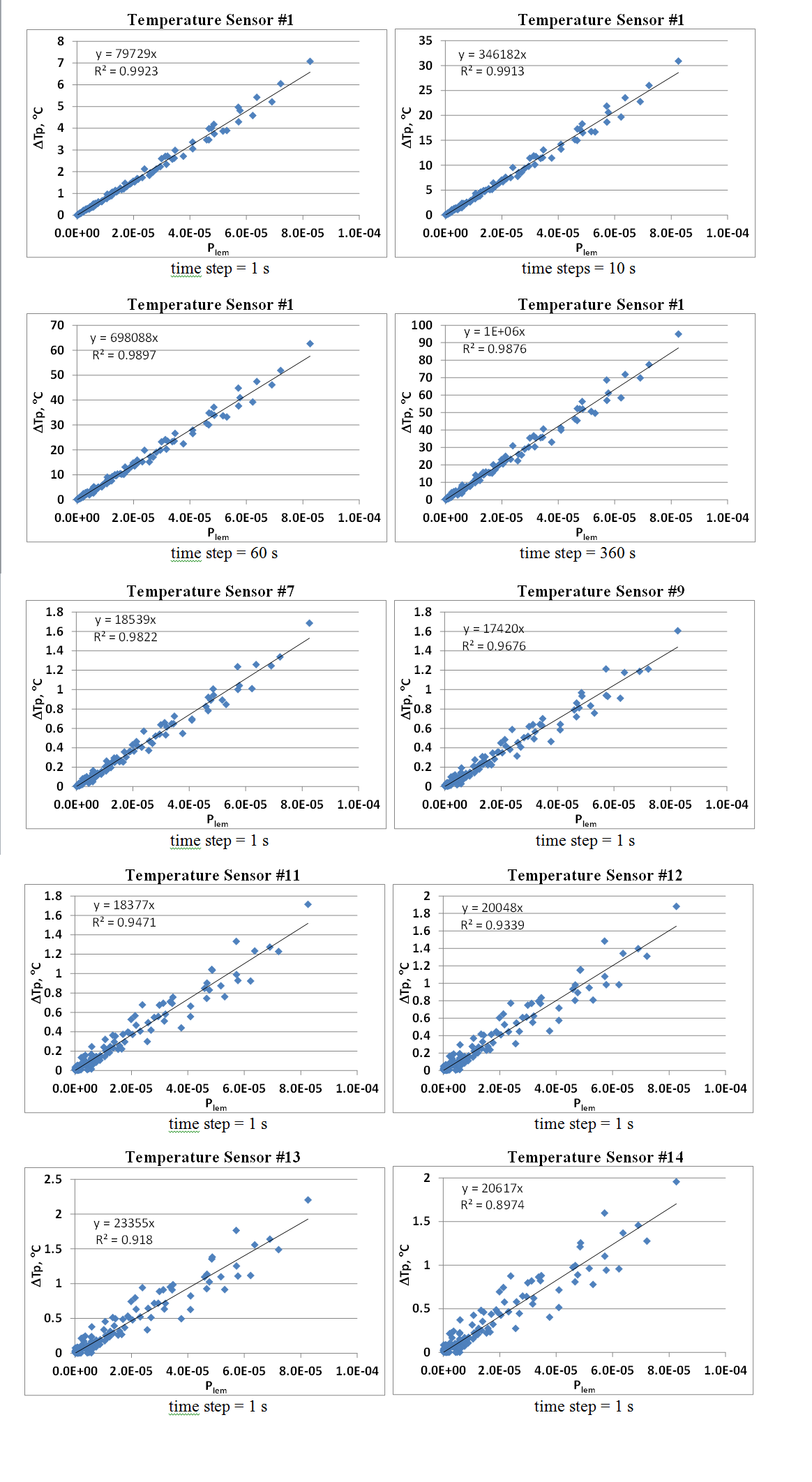
Our test objects were titanium alloy helix and straight wire insulated lead (Fig. 1). The leads were positioned in the middle of a box filled with a medium with εr=78 and σ=1.2S/m. 120 Etan(l) along the lead trajectory was generated by four antennas located along one side of the box by varying the relative antenna positions as well as the amplitude and the phase of each antenna source. P was calculated by integrating the volume loss density (VLD) around the lead tip. Additionally point VLD values (VLD3D_EM) were obtained at axial location 1mm from the tip. S(l) for the tip electrode was calculated using the reciprocity approach described in [3]. 3D-EM simulations were performed at 127.7MHz using ANSYS HFSS-2014 (ANSYS, Canonsburg, USA). 3D temperature distributions after 1, 10, 60, 360 and 900 seconds continuous excitation were calculated using the ANSYS-15. ΔTp was obtained at 14 locations. The variable mesh was generated in each solver independently. The mesh size in the area of the hot spot was less than 0.1 mm. The 3D-EM mesh adaptation procedure with 30% increase of the mesh elements was stopped if the variation of P or ‖S‖max between two consecutive meshes was less than 3%. The convergence of the thermal simulations was obtained by the manual reduction of the mesh size between two consecutive runs of the thermal solver for a given 3D-EM simulation. The mesh reduction was stopped when the difference between maximum induced temperature rise (ΔTmax) of two consecutive runs was less than 3%.Results and Discussion:
Variation of antenna location, source amplitudes, and phases is a robust approach to generate different amplitude and phase distributions. R2A was 0.9714 and 0.5759 for straight and helix lead, respectively. The latter means that this linear regression was rather poor. However the linear regression for VLD3D_EM was very good: 0.9876. Thus the LEM can predict VLD at axial locations 1mm from the helix lead tip. This was strong evidence of the reliable calculation of TF for straight and helix leads. For helix lead diversity of the pathways influenced on both VLD and temperature distribution. For the helix lead R2ATp depended substantially on the duration of the RF-induced heating and also significantly on the location of temperature probe. For the straight lead the influence of R2(ATp) on the location of temperature probe was significantly smaller but still noticeable. The ratio AVLD/A was equal 5.98 and 12.33 for straight and helix leads, respectively. It provided strong evidence that power deposition distribution depends not only on lead tip geometry and the surrounding medium, but also on lead wire geometry.Conclusion:
LEM was a suitable approach for predicting VLD or temperature in close proximity to the end face of lead tip. However for the helix lead the variance of the fitted values and observed values was rather high for ATp at other locations around the lead tip as well as for A. The variation of the power deposition and the RF-induced heating profiles in the proximity of the lead tip due to Etan(l) cannot be readily generalized to the wider range of lead geometries and tissue dielectric properties, because we investigated only one set of Etan(l), two lead geometries, and only one set of tissue dielectric properties.Disclaimer:
The mention of commercial products, their sources, or their use in connection with material reported herein is not to be construed as either an actual or suggested endorsement of such products by the Department of Health and Human Services.Acknowledgements
No acknowledgement found.References
[1] Technical specification ISO/TS 10974, “Assessment of the safety of magnetic resonance imaging for patients with an active implantable medical device”, 1st edition 2012.
[2] S-M. Park, K. Kamondetdacha, and J. A. Nyenhuis, “Calculation of MRI-induced heating of an implanted medical lead wire with an electric field transfer function”, J. Magn. Reson. Imaging, 26(5), 2007, 1278–1285.
[3] S. Feng, R. Qiang, W. Kainz, and J. Chen, “A technique to evaluate MRI-Induced electric fields at the ends of practical implanted lead,” IEEE Transactions on Microwave Theory and Techniques, 63(1), 2015, 305-313.
Figures