3939
In Search of Repeatable and Useful Prostate DCE1Brigham and Women's Hospital, Boston, MA, United States
Synopsis
This work aims to improve the practical utility of DCE derived quantitative biomarkers by comparing the repeatability of DCE calculated parameters across analysis methods, and across AIF choices. The data consists of two scans each from a set of 15 patients with suspected prostate cancer, repeated within 14 days without intervening therapy.
INTRODUCTION
There is wide consensus that quantitative DCE could have a role as a surrogate marker for disease recurrence and for evaluation of response to neoadjuvant drug therapy1,2,3. However, modeling and analysis of DCE is disappointingly notable for the variability of calculated parameters - both between patients and between studies. A major criterion for a useful biomarker is knowledge of an accepted degree of variability in quantitative indices between two scans without intervening therapy. One of the major sources of variability in DCE calculations is the uncertainty involved in determining the arterial contrast agent time-dependent concentration curve, also called the arterial input function (AIF)4.
This work sets out to improve the practical utility of DCE derived quantitative biomarkers by comparing the repeatability of DCE calculated parameters across analysis methods, and across AIF choices. Each of the methods and AIF choices investigated here was also evaluated for its discriminatory ability between a prostate peripheral zone area of suspected malignancy and an area categorized as healthy.
METHODS
As part of a multiparametric MRI repeatability study 5, two clinical prostate DCE scans were performed on 15 treatment-naïve patients within an interval of less than two weeks on a 3T scanner using an endorectal coil (Figure 1). Left and right femoral artery voxels were segmented for AIF measurement (designated ‘LA’ and ‘RA’ in figures), as were tumor-suspicious regions and normal tissue in the peripheral zone (‘TPZ’ and ‘NPZ’ respectively - see Figure 2). A semi-automated method of finding an ROI from which to estimate the AIF was also implemented (‘MY’ in the figures) to check whether standardization of the process of identifying the AIF could remove some operator-induced variability. Another AIF which consisted of the population average of all other AIF’s was also applied (‘MN’).
If the AIF is measured in a large artery upstream from the tissue of interest, further downstream the concentration may be delayed. Here we attempt to correct for a possible shift in the bolus arrival time (BAT). Ignoring BAT has been shown to degrade the fit quality in DCE modeling 6, while incorporation of a BAT shift has shown improved reproducibility of calculated model parameters 7. The analysis methods evaluated were:
- Two parameter Tofts yielding Ktrans and ve 8,9;
- Three parameter Extended Tofts yielding Ktrans, ve, and vp 10;
- Two parameter Tofts with BAT fitting;
- Three parameter Tofts with BAT fitting.
Hematocrit was estimated at 0.45; arterial T1 of blood was always taken as 1630 ms 11 and tissue T1 was assumed constant at 1434 ms 12.The parameters Ktrans, ve, and vp (for the 3 parameter models) were calculated for each voxel in the ROIs TPZ and NPZ, and then averaged over the ROI.
In order to rank the methods according to repeatability, the absolute percent difference between of all pairs of repeated measures in the TPZ and the NPZ was calculated for all methods - referred to as the mean absolute percent difference (MAPD). Discrimination between the parameter values in the ROI’s TPZ and NPZ was assessed by a paired t-test on all the scans, one-tailed for Ktrans and vp, and two-tailed for ve.
RESULTS
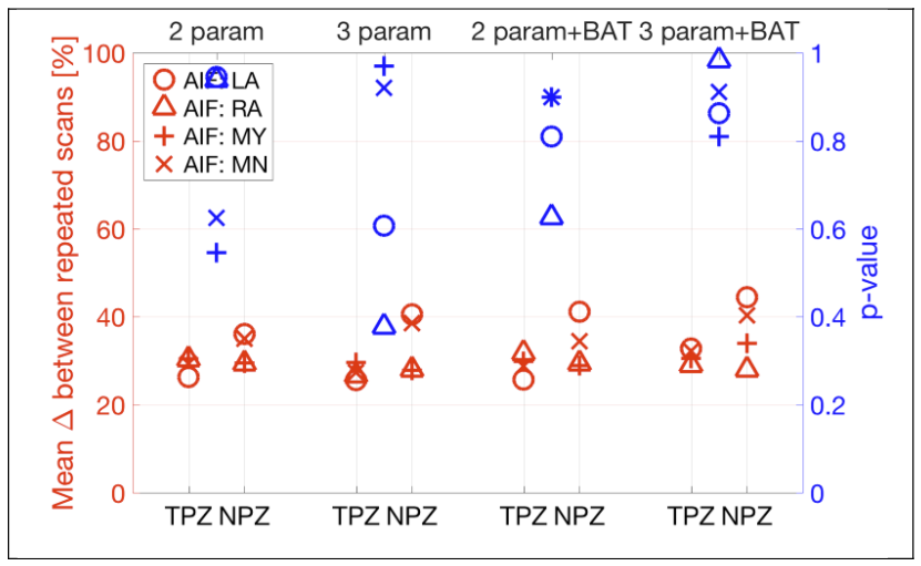
Figure 3 shows that the Ktrans MAPD was between 30-40% for TPZ and worse (higher) for NPZ. The addition of BAT fitting improved Ktrans MAPD values slightly. Differentiation of TPZ and NPZ was good, with p<0.05 for right artery AIF, for all analyses except 3 parameter+BAT.
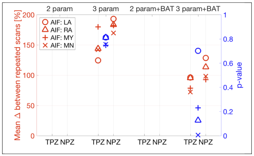
Figure 4 shows that MAPD for ve was generally better than for Ktrans, but discrimination between TPZ and NPZ was minimal for ve. Addition of BAT fitting to the analysis did not seem to affect the results for ve.
Figure 5 shows that in the case of vp, a drastic improvement in both MAPD repeatability and tumor discrimination was obtained by adding BAT to the fitting model, with p<0.005 when using the mean AIF (MN).
The best overall AIF for repeatability was that derived from the right artery ROI (RA)
DISCUSSION AND CONCLUSIONS
While prostate DCE repeatability is challenging, it is important to determine the best methods for rendering clinical data usable for treatment response studies. Additional non-Tofts analysis techniques could also be applied and compared. Here, addition of BAT fitting was beneficial for vp repeatability and tumor discrimination but did not substantially affect those measures for Ktrans and ve. The use of a mean function as the AIF was not an advantage, and neither was the semi-automated AIF derivation. The parameters in the normal tissue ROI were consistently less repeatable than in the tumor ROI. Our plan is to next apply the improved understanding of DCE analysis repeatability as part of a response assessment study in patients that underwent combination neoadjuvant and radiation therapy.Acknowledgements
NIH U24 CA180918, P41 EB015898, U01 CA151261.
References
1. Barrett, T. et al. DCE and DW MRI in monitoring response to androgen deprivation therapy in patients with prostate cancer: a feasibility study. Magn. Reson. Med. 67, 778–785 (2012).
2. Alic, L. et al. Heterogeneity in DCE-MRI parametric maps: a biomarker for treatment response? Phys. Med. Biol. 56, 1601–1616 (2011).
3. Sung, Y. S. et al. Dynamic contrast-enhanced MRI for oncology drug development. J. Magn. Reson. Imaging 44, 251–264 (2016).
4. Sourbron, S. P. & Buckley, D. L. Classic models for dynamic contrast-enhanced MRI. NMR Biomed. 26, 1004–1027 (2013).
5. Fedorov, A., Vangel, M. G., Tempany, C. M. & Fennessy, F. M. Multiparametric Magnetic Resonance Imaging of the Prostate: Repeatability of Volume and Apparent Diffusion Coefficient Quantification. Invest. Radiol. 52, 538–546 (2017).
6. Mehrtash, A. et al. Bolus arrival time and its effect on tissue characterization with dynamic contrast-enhanced magnetic resonance imaging. J Med Imaging (Bellingham) 3, 014503 (2016).
7. Chouhan, M. D. et al. Estimation of contrast agent bolus arrival delays for improved reproducibility of liver DCE MRI. Phys. Med. Biol. 61, 6905–6918 (2016).
8. Kety, S. S. The theory and applications of the exchange of inert gas at the lungs and tissues. Pharmacol. Rev. 3, 1–41 (1951).
9. Tofts, P. S. & Kermode, A. G. Measurement of the blood-brain barrier permeability and leakage space using dynamic MR imaging. 1. Fundamental concepts. Magn. Reson. Med. 17, 357–367 (1991).
10. Tofts, P. S. et al. Estimating kinetic parameters from dynamic contrast-enhanced T(1)-weighted MRI of a diffusable tracer: standardized quantities and symbols. J. Magn. Reson. Imaging 10, 223–232 (1999).
11. Lu, H., Clingman, C., Golay, X. & van Zijl, P. C. M. Determining the longitudinal relaxation time (T1) of blood at 3.0 Tesla. Magn. Reson. Med. 52, 679–682 (2004).
12. Fennessy, F. M. et al. Practical considerations in T1 mapping of prostate for dynamic contrast enhancement pharmacokinetic analyses. Magn. Reson. Imaging 30, 1224–1233 (2012).
13. Fedorov, A. et al. 3D Slicer as an image computing platform for the Quantitative Imaging Network. Magn. Reson. Imaging 30, 1323–1341 (2012).
Figures
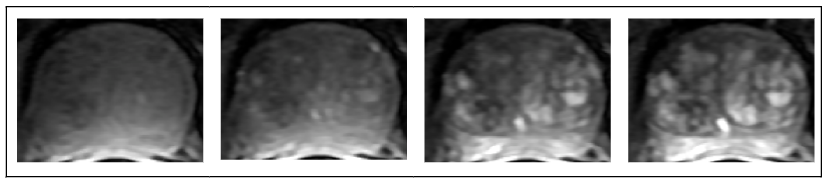
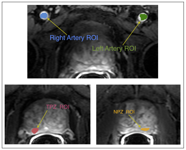
Figure 2. Examples of the Regions of Interest (ROIs) that were identified and segmented by an experienced abdominal radiologist on each DCE image:
- Peripheral zone tumor-suspicious ROI (TPZ) (tumor was identified in 11 patients only);
- One normal-appearing peripheral zone ROI (NPZ);
- Left artery voxels (LA) for AIF measurement;
- Right artery voxels (RA) for AIF measurement.
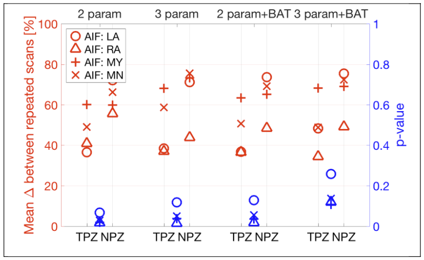
Figure 3. Ktrans repeatability and tumor discrimination for different AIFs and analysis methods.
In red (left axis), is the average of the % differences between repeated scans for AIFs from Left Artery ROI (LA); Right Artery ROI (RA); Semi-automated segmentation of blood voxels AIF (MY); and using the mean AIF of the group (MN).
In blue (right axis), p-values from paired one-sided t-tests comparing $$$K_{trans}$$$ in peripheral zone tumor-suspicious ROI (TPZ) and normal peripheral zone ROI (NPZ).