Synopsis

We propose a machine-learning framework for brain temperature estimation in MRSI using human in-vivo data from 1.5T and 3T scanners. We consider the chemical-shift based method as our benchmark and compare our results against it. Our framework, based on random-forest regression, performs a K-fold cross validation on the MRSI dataset which includes (1) learning the spectral features (including the chemical-shift) from the subjects; (2) obtaining brain temperature estimates and computing the error over the corresponding jMRUI-fitted chemical-shift based estimates. Compared to jMRUI, our method, after training, gives a low estimation error and a 30-fold improvement in estimation speed per patient.

Introduction

Methods

Random Forests⁵ have been used in MRSI towards classification^6-7 and quantification⁸ of spectral data. These involve multiple forests comprising of a set of binary trees. For training, splits are created in each tree based on random subsets of the feature variables and piecewise linear regression is performed over the input data. The process involves seeking best prediction at every node and using thresholding to further propagate data points till they reach the end of the tree. Subsequently the weighted average of the prediction from each tree is taken to give a single output estimate.

Subjects. 10 healthy, male volunteers in the age range of 23-40 years (mean +/- SD, 30.5 +/- 5.2 years) were invited for scanning on 3 occasions and underwent 4 MRSI scans each on both 1.5T (PRESS sequence, TR/TE = 1000/144ms, FOV = 300mm², 24-step phase encoding in both in-plane directions) and 3T (semi-LASER PRESS sequence, TR/TE = 1700/144ms, FOV = 256mm²) scanners during each visit. Data was zero-filled (in k-space), interpolated to 32x32 voxels and corrected for eddy-and phase-correction. Additional details can be found in [1]. Data-fitting was done using the AMARES algorithm⁹ and voxels with poor quality of NAA-fits and water-resonance distortions were rejected. Total spectra per fold included approximately $$$\textbf{1800}$$$ training and $$$\textbf{150}$$$ test-spectra/subject respectively.

In MRSI, the time-domain complex signal of a nucleus is given by: $$S(t) = \int \mathrm{p}(\omega)\mathrm{exp}(-i\Phi)\mathrm{exp}(-t/T^{*}_{2})d\omega$$,

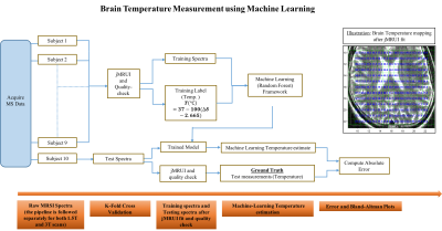
and the corresponding frequency-domain spectrum is given by $$$S(\omega)$$$. As shown in Fig.1, we aim to perform the inverse signal modeling where we have a training dataset $$$D = (S_{i} (\omega), T_{i}), i\in [1, N]$$$, where $$$N$$$ is the total number of training spectra from 9 subjects.

$$$S_{i}(\omega)$$$ represents the training data. $$$T_{i}$$$ are the training-labels which correspond to the temperature evaluated using the chemical-shift method¹. To ensure data-homogeneity, we train spectra that pass the quality-control measure post-fitting. Using the dataset from each scanner, we perform a separate K-fold cross validation comprising 10 folds (each having $$$\textbf{100}$$$ trees and mTry = $$$\textbf{128}$$$). Each fold comprises of a training-set from 9 subjects and test-spectra, $$$S_{j}(\omega)$$$, from the remaining subject to obtain the brain temperature estimates $$$\hat{T}_{j}$$$. The corresponding chemical-shift based temperature-estimates $$$T_{j}$$$ serve as the ground-truth, $$$j\in [1, M]$$$ where $$$M$$$ is the total number of test spectra.

Error Calculation. For our experiments, given the estimate $$$\hat{T}_{j}$$$ and the test temperature $$$T_{j}$$$ for a given subject, the estimate error $$$\hat{E}_{j}$$$ (in $$${^\circ}C$$$) can be calculated as, $$\hat{E}_{j} = ||\hat{T}_{j} - T_{j}||_{1}$$

Results

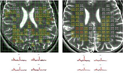
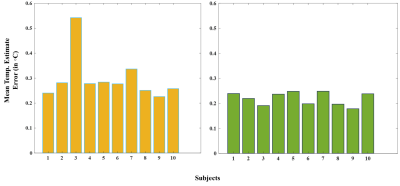
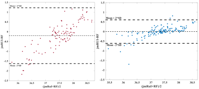
The temperature-mapping estimates for a sample subject using both the chemical-shift and the random-forest (RF) methods have been shown in Fig.2, and the corresponding Bland-Altman plots¹⁰ for the same subject also show a strong correlation (Fig.4). The mean relative-error plots for each subject is shown in Fig.3.

Speed: Training time-per-fold is 1 minute. While the jMRUI-fitting takes 5 minutes per subject for approximately 150 spectra, our proposed framework, after training, takes only 10 seconds leading to a $$$\textbf{30x}$$$ improvement in speed.

Discussion and Conclusion

In Fig.2, the temperature difference between the 2 methods are minimal leading to a low-error. A slightly higher-error can be seen around the edges and CSF regions possibly due to variations in spectral-pattern in these areas. Such spectra are fewer in number (post quality-check) and therefore the framework is insufficiently trained to identify similar spectral-patterns. The outliers observed in the corresponding Bland-Altman plots (Fig.4) belong to these regions. The RF-method tends to slightly overestimate temperatures relative to jMRUI at the lower end of the (jMRUI) temperature-range.

The mean-error plots (Fig.3) correspond to an overall mean error of $$$\textbf{0.29} {^\circ}C$$$ for the 1.5T data and $$$\textbf{0.20} {^\circ}C$$$ for the 3T data (due to better spectral-quality and resolution). Estimates for Subject 3 exhibited a slightly higher error for the 1.5T data but this issue wasn't present while evaluating the corresponding 3T data.

Future Work

Acknowledgements

References

[1] Thrippleton, M.J., Parikh, J., Harris, B.A., Hammer, S.J., Semple, S.I.K., Andrews, P.J.D., Wardlaw, J.M., Marshall, I.: Reliability of mrsi brain temperature mapping at 1.5 and 3 t. NMR in Biomedicine 27(2), 183-190 (2014).

[2] Kuroda, K., Suzuki, Y., Ishihara, Y., Okamoto, K., Suzuki, Y.: Temperature mapping using water proton chemical shift obtained with 3d-mrsi: Feasibility in vivo. Magnetic Resonance in Medicine 35(1), 20-29 (1996).

[3] Parker, D.L.: Applications of nmr imaging in hyperthermia: An evaluation of the potential for localized tissue heating and noninvasive temperature monitoring. IEEE Transactions on Biomedical Engineering BME-31(1), 161-167 (Jan 1984).

[4] Bihan, D.L., Delannoy, J., Levin, R.L.: Temperature mapping with mr imaging of molecular diffusion: application to hyperthermia. Radiology 171(3), 853-857 (1989).

[5] Breiman, L.: Random forests. Machine Learning 45(1), 5-32 (2001).

[6] Pedrosa de Barros, N., McKinley, R., Wiest, R., Slotboom, J.: Improving labeling efficiency in automatic quality control of mrsi data. Magnetic Resonance in Medicine (2017).

[7] Menze, B.H., Kelm, B.M., Weber, M.A., Bachert, P., Hamprecht, F.A.: Mimicking the human expert: Pattern recognition for an automated assessment of data quality in mr spectroscopic images. Magnetic Resonance in Medicine 59(6), 1457-1466 (2008).

[8] Das, D., Coello, E., Schulte, R.F., Menze, B.H.: Quantification of Metabolites in Magnetic Resonance Spectroscopic Imaging Using Machine Learning, pp. 462-470. Springer International Publishing, Cham (2017).

[9] Stefan, D., Cesare, F.D., Andrasescu, A., Popa, E., Lazariev, A., Vescovo, E., Strbak, O., Williams, S., Starcuk, Z., Cabanas, M., van Ormondt, D., Graveron- Demilly, D.: Quantitation of magnetic resonance spectroscopy signals: the jmrui software package. Measurement Science and Technology 20(10), 104035 (2009).

[10] Bland, J.M., Altman, D.: Statistical methods for assessing agreement between two methods of clinical measurement. The Lancet 327(8476), 307-310 (1986).