3837
Multi-exponential T2* mapping distinguishes benign/malignant lymph nodes in rectal cancer patients: an ex-vivo and in-vivo experiment1Radiology Department, Champalimaud Research, Champalimaud Centre for the Unkown, Lisbon, Portugal, 2Computational Clinical Imaging Group, Champalimaud Research, Champalimaud Centre for the Unkown, Lisbon, Portugal, 3Neuroplasticity and Neural Activity Lab, Champalimaud Research, Champalimaud Centre for the Unkown, Lisbon, Portugal, 4Centre for Medical Imaging Computing, Department of Computer Science, University College London, London, United Kingdom
Synopsis
In rectal cancer patient management, quality-of-life compromise due to unnecessary neoadjuvant chemoradiation is a major concern and may be driven by false positive lymph node(LN) staging. We sought to distinguish benign LNs from LNs with different patterns of malignant infiltration by investigating multi-exponential decay in multi-gradient-echo(MGE) MRI ex-vivo, at 16.4T. The experiment was translated to the clinic and performed at 1.5T during rectal cancer staging. We found that the 2-compartment model of T2* decay allows malignant and benign LNs to be distinguished in clinical images with a higher specificity than that of conventional criteria, namely short-axis>5mm, border irregularity and mixed signal intensity.
INTRODUCTION
Lymph node(LN) staging is essential in rectal cancer patient´s management, yet current implemented imaging methods show limited accuracy for that purpose1. Multigradient echo(MGE) MRI was used with a mono-exponential signal decay model for investigating LNs in breast cancer2,3. It was also explored for LN characterization in colorectal cancer using a multi-exponential approach4. This study explores MGE-derived compartment-specific information in LNs retrieved from rectal cancer specimens, as well as in patients in-vivo using nonlinear characteristics of MGE signal decay. Our findings show that MGE differentiates benign LNs from LNs with different patterns of malignant infiltration and may thus assist in LN staging.METHODS
Institutional setting, approved by ethics committee
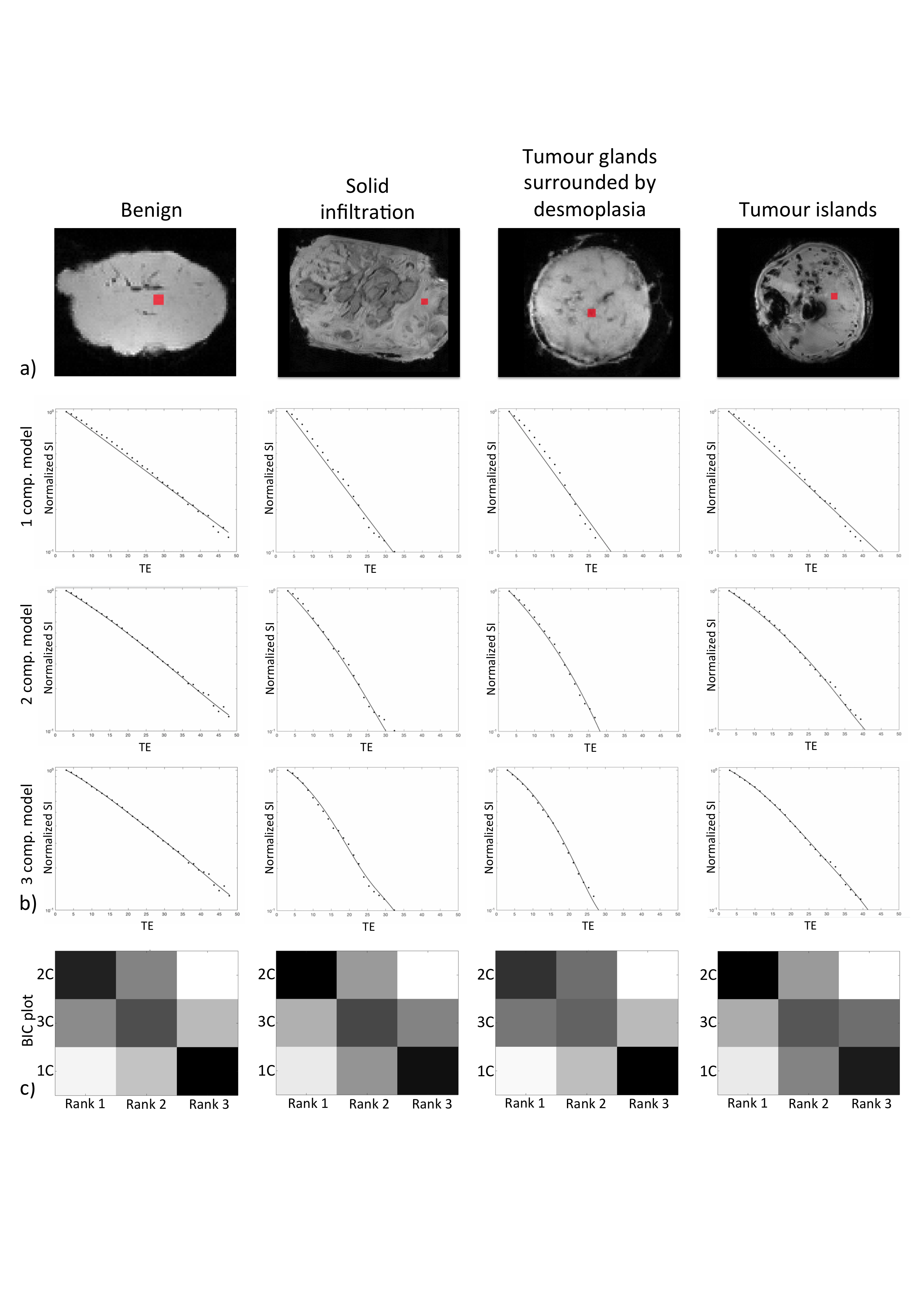
Ex-vivo experiment: 33 benign and 32 malignant LNs with different infiltration patterns [tumour glands surrounded by desmoplasia(n=20), tumour islands(n=6), solid infiltration(n=6)] were retrieved from surgical specimens of 11 consecutive N+ rectal cancer patients(mean age=61.6y, 5 males), preserved in 4% formaldehyde and moved to 1% PBS 24h before scanning.
In vivo experiment: Eight consecutive patients with rectal cancer underwent a MGE acquisition during staging pelvic MRI on a 1.5T clinical scanner. Six underwent total mesorectal excision without neoadjuvant therapy and were considered eligible(mean age:61,7y; 4 males). Mapping during specimen processing allowed 36 benign and 27 malignant LNs to be matched to MGE images.
Image acquisition
Ex-vivo experiment: Retrieved LNs were immersed in Flourinert® within an NMR tube. Images were acquired at 37ºC in a 16.4T Bruker Ascend Aeon scanner using a Micro5 NMR imaging probe. A fat-suppressed MGE sequence was applied: 50 TEs starting at 1.6ms with 1.4ms interval, TR=1500 ms, FA=50º; ST=0.3mm; in-plane resolution=(0.1 mm)2, Bandwidth=125000Hz; 25 averages.
In-vivo experiment: A MGE acquisition was performed: 32 TEs starting at 2.37ms with 2.37ms interval, TR=1519ms, FA=55º, ST=4mm; in plane resolution=(0.42mm)2, Bandwidth=431,3 Hz, 2 averages.
Data analysis
Magnitude signal was fitted using 1-, 2- and 3-compartment T2* models. In multi-compartment models, one compartment is arbitrarily assumed on-resonance, while others exhibit a frequency shift. Signal expressions:
S1C(TE)=S0exp(-TE/T2*)
S2C(TE)=S0|f1exp(-TE/T2*a)+(1-f1 )exp(-TE(1/T2*b )+i∆ω)|
S3C(TE)=S0|f1exp(-TE/T2*1)+f2exp[-TE(1/T2*2)+i∆ω1]+(1-f1-f2)exp[-TE(1/T2*3)+i∆ω2] |
TE=echo time; S0=signal at TE=0; T2*i=relaxation time of compartment i with volume fraction fi and frequency shift ∆ωi.
Ex-vivo experiment: MR datasets up to 34th TE were smoothed in k-space and analyzed in Matlab®. Models were fitted voxel-wise using constrained non-linear optimization accounting for Rician noise.
In-vivo experiment: Whole-node ROIs were defined manually on a single slice. MR datasets up to TE=40ms were considered and models were fitted to the ROI median of each LN using constrained non-linear optimization accounting for Rician noise.
Models were compared based on Bayesian Information Criterion(BIC). Then, histogram analysis was performed for the model parameters. Finally, receiver operating characteristics(ROC) were computed.
Statistical analysis
Median values were used (data not normally distributed). Comparison between benign and malignant LNs was performed using Mann-Whitney U test. For the ex-vivo experiment, benign and malignant LN subgroups were compared using Kruskal-Wallis test to account for multiple comparisons.
RESULTS
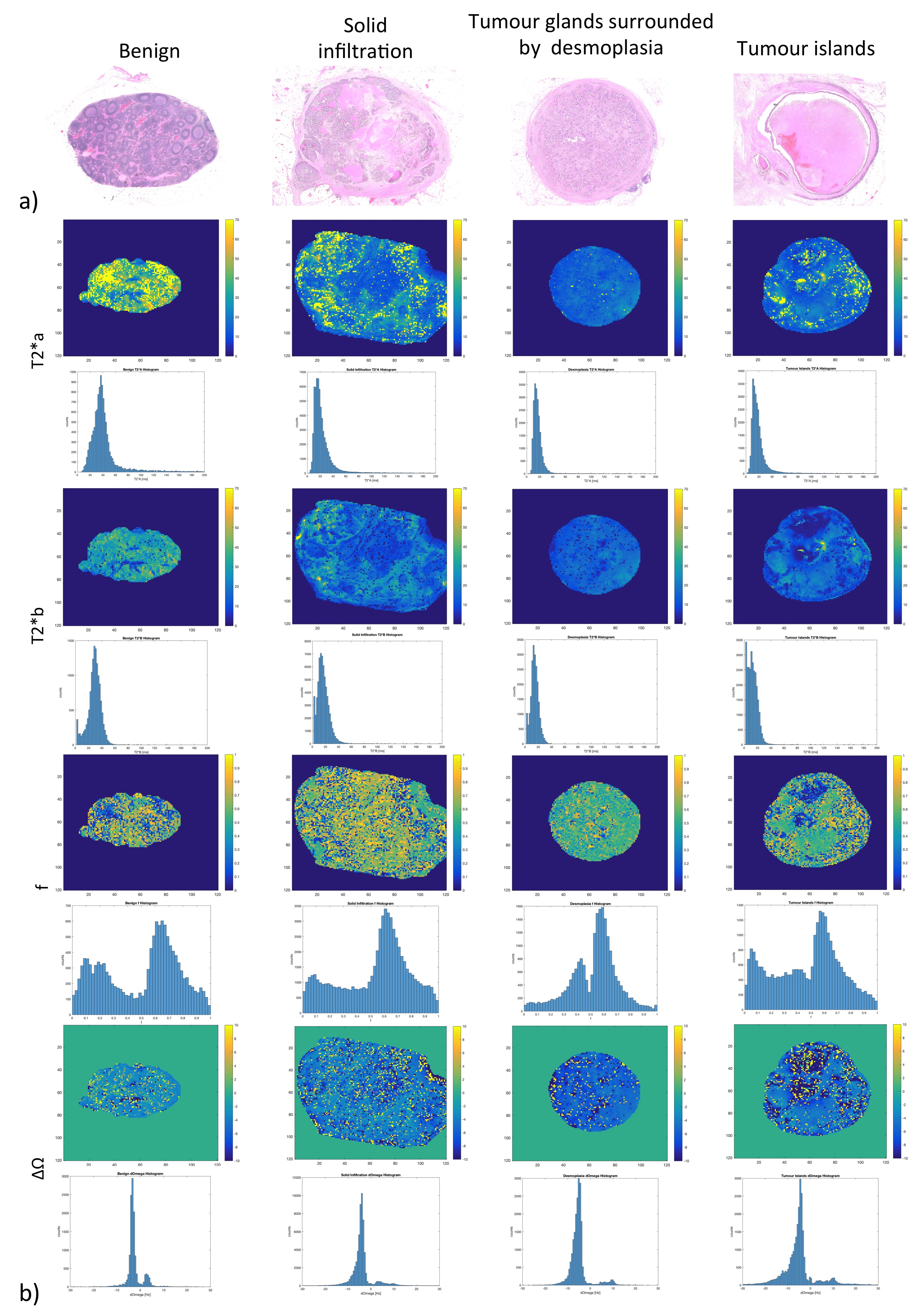
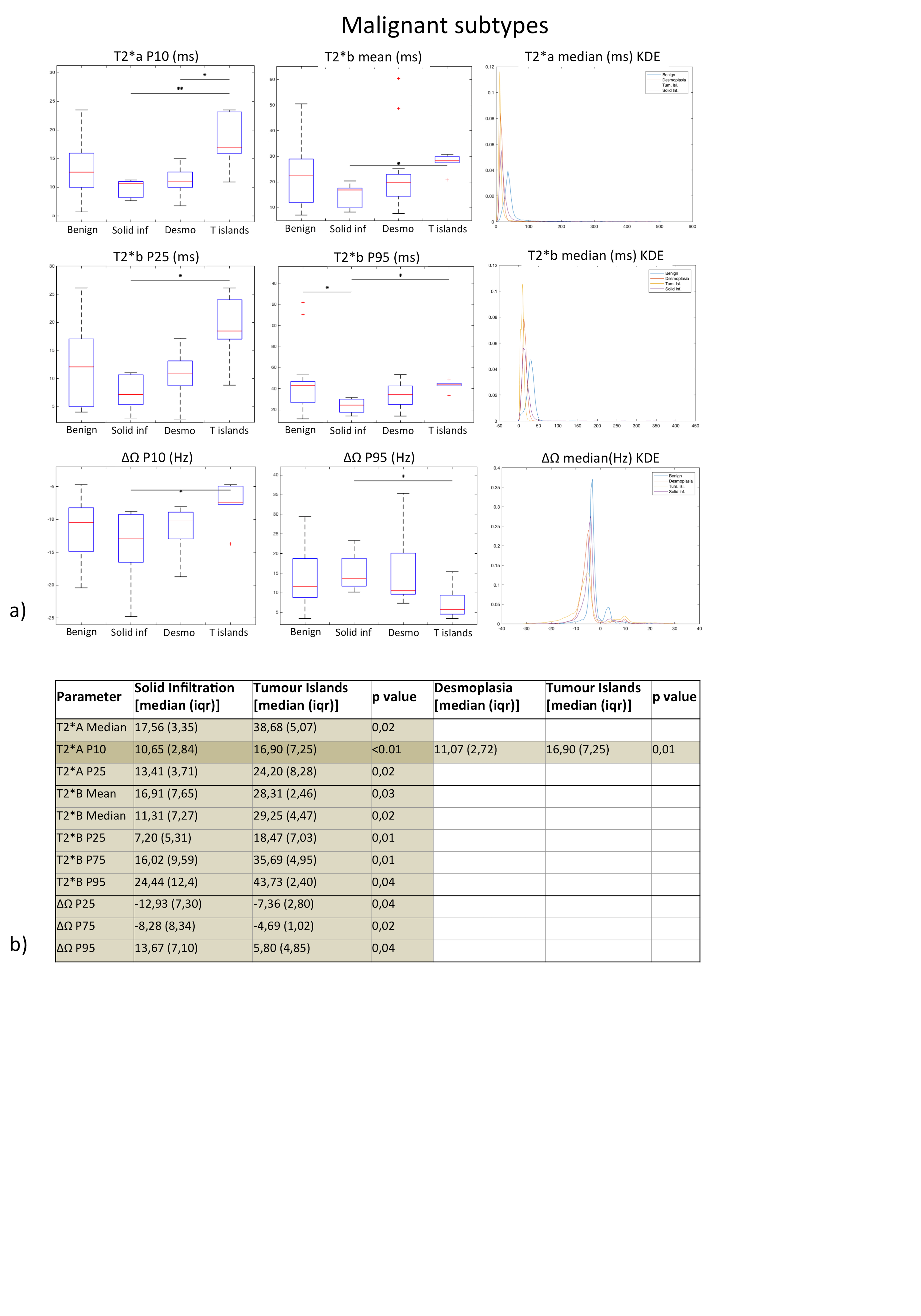
Ex-vivo experiment: Figure 1 shows examples of data fits of our 3 models for each LN category(1b) and corresponding BIC-based model ranking for whole-node VOIs(1c). The 2-compartment model(2-cm) ranked first in most instances. Figure 2 depicts histologic characteristics(2a), parameter maps and histograms of the voxel-wise fit for 2-cm(2b). Figure 3 shows boxplots of the most discriminative parameters, including histogram metrics; and kernel density estimation(KDE)(3a). Median, iqr and p values of each parameter(bounded parameters excluded) are displayed in 3b. ROC curves in 3c compare 1-cm and 2-cm when the best significant metric from each parameter is combined. A similar analysis for different LN subtypes is given in Figure 4.
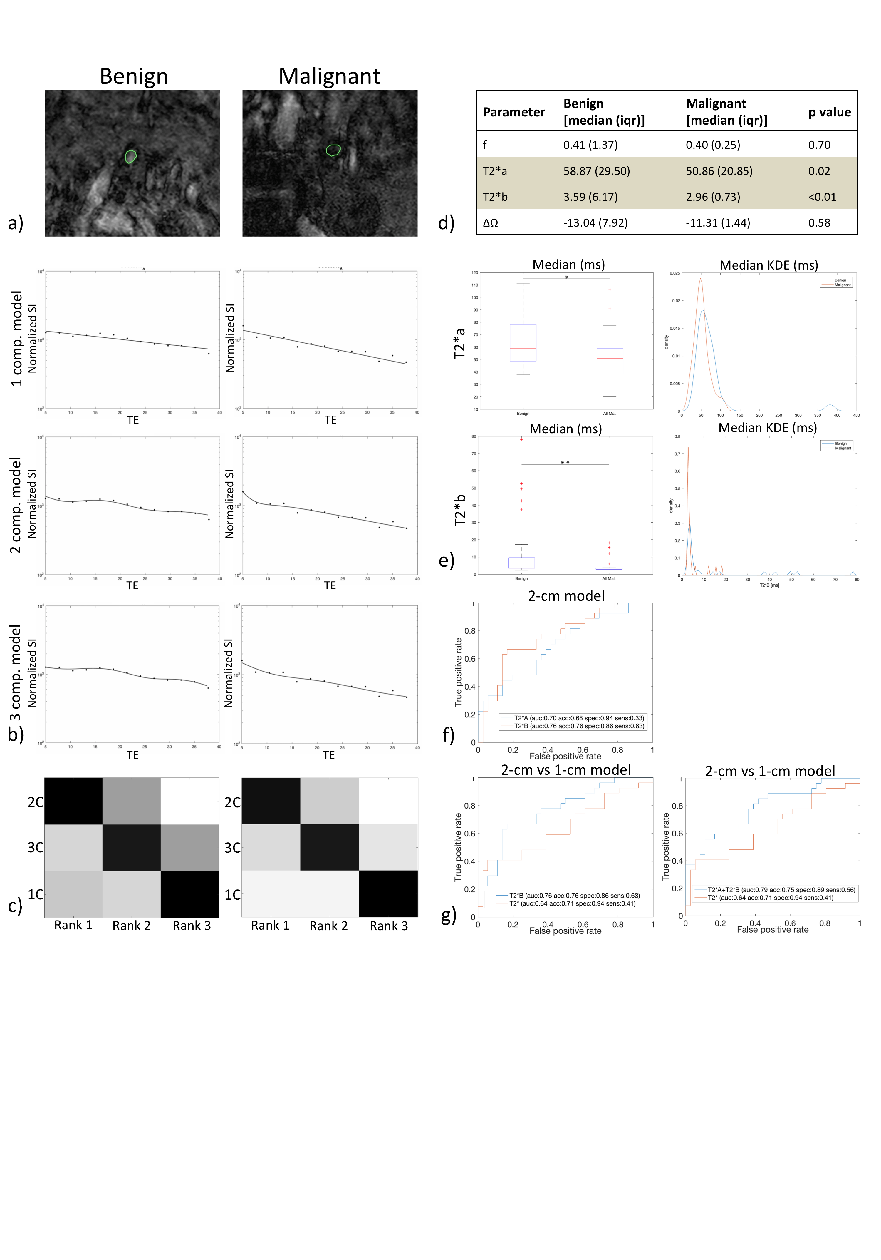
In vivo experiment: Data fits of the 3 models(5b) and BIC-based model ranking(5c) for whole-node ROIs again suggested 2-cm’s superiority. Median, iqr and p values of the parameters are displayed in 5d, while boxplots and KDE are given in 5e. 5f shows ROC curves for T2*a and T2*b(2-cm) while 5g compares ROC curves for the best performing parameters of 1-cm and 2-cm.
DISCUSSION
Significant differences between malignant and benign LNs were found in several metrics derived from T2*a, T2*b, f and ∆Ω. The single most discriminative parameter was kurtosis of f. In-vivo at 1.5T, T2*a also presented significantly higher values in benign LN and displayed a high specificity for malignancy (0.94). T2*b showed a higher discriminative power with an auROC of 0.76 and specificity of 0.86. The performance of the 2-cm exceeded that of the 1-cm (auROC=0.79vs0.64, respectively). The specificity of T2*a, T2*b and of their combination (2-cm) exceeded that of conventional imaging criteria such as short axis>5mm, border irregularity and mixed signal intensity5,6.CONCLUSION
Our results indicate multi-compartment T2* mapping may be of added value for LN staging in rectal cancer.Acknowledgements
This study was supported by funding from the Champalimaud Foundation (project number 132) and from the Engineering and Physical Sciences Research Council (EPSRC), grant number M507970.
We would like to acknowledge:
António Beltran, MD, PhD, Pathology Department, Champalimaud Centre for the Unknown, Lisbon, Portugal
António Galzerano, MD, Pathology Department, Champalimaud Centre for the Unknown, Lisbon, Portugal
Alexandra Martins, Pathology Department, Champalimaud Centre for the Unknown, Lisbon, Portugal
Lara Castanheira, Pathology Department, Champalimaud Centre for the Unknown, Lisbon, Portugal
Joana Maia, Systems Oncology Lab, Champalimaud Research, Champalimaud Centre for the Unknown, Lisbon, Portugal
Bruno Costa da Silva, PhD, Systems Oncology Lab, Champalimaud Research, Champalimaud Centre for the Unknown, Lisbon, Portugal
Nuno Loução, Philips Iberia, Philips Healthcare
Paula Montesinos, Philips Iberia, Philips Healthcare
Javier Sanchez-Gonzalez, Philips Iberia, Philips Healthcare
Rita Theias, MD, Pathology Department, Hospital Fernando Fonseca EPE, Lisbon, Portugal
Carlos Leichsenring, MD, Surgery Department, Hospital Fernando Fonseca EPE, Lisbon, Portugal
Vasco Geraldes, MD, Surgery Department, Hospital Fernando Fonseca EPE, Lisbon, Portugal
References
(1) Bipat S, Afina GS, Slors FJM, Zwinderman AH, Bossuyt PMM, Stoker J. Rectal Cancer: Local Staging and Assessment of Lymph Node Involvement with Endoluminal US, CT, and MR Imaging—A Meta-Analysis. Radiology 2004; 232:773–783.
(2) Korteweg MA, Zwanenburge JJM, Hoogduin JM, van der Bosch AAJ, van Diest PJ, van Hillegersberg R, Eijkemans JC et al. Dissected sentinel lymph nodes of breast cancer patients: characterization with high-spatial-resolution 7-T MR imaging. Radiology. 2011. 261: 127-135.
(3) Li C, Meng S, Yang X, Wang J and Hu J. The value of T2* in differentiation metastatic from benign axillary lymph nodes in patients with breast cancer – a preliminary in vivo study. PloS One. 2014. 9(1):e84038.
(4) Santiago I, Ianus A, Matos C, Shemesh N. Characterization of lymph nodes in colorectal cancer using non-exponential modeling of T2* decay [abstract]. In: 25th Annual Meeting & Exhibition; 2017 Apr 22-27; Honolulu, HI, USA: ISMRM; 2017. Abstract nr 4503.
(5) Doyon F, Attenberger UI, Dinter DJ, Schoenberg SO, Post S, Kienle P. Clinical relevance of morphologic MRI criteria for the assessment of lymph nodes in patients with rectal cancer. Int J Colorectal Dis. 2015; 11:1541-1546.
(6) Brown G, Richards CJ, Bourne MW, Newcombe RG, Radcliffe AG, Dallimore NS, Williams GT. Morphologic predictors of lymph node status in rectal cancer with use of high-spatial-resolution MR imaging with histopathologic comparison. Radiology. 2003 May;227(2):371-7
Figures