3560
Multichannel Hyperpolarized 13C MRI in a Patient with Liver Metastases using Multi-slice EPI and an Alternating Projection Method for Denoising1Department of Electrical Engineering, Technical University of Denmark, Kgs. Lyngby, Denmark, 2Department of Radiology and Biomedical Imaging, UCSF, San Francisco, CA, United States, 3UC Berkeley-UCSF Graduate Program in Bioengineering, UC Berkeley and UCSF, San Francisco, CA, United States, 4Department of Medicine, UCSF, San Francisco, CA, United States
Synopsis
Hyperpolarized 13C-pyruvate for monitoring metabolism of liver metastases in vivo is being investigated for clinical trials of new therapeutics. This study applied advances in multichannel receive arrays and sequence design for human 13C liver imaging and investigated a new denoising method. The method is based on an alternating projection method to enforce structuredness and low-rankness, and is applied with automatic threshold estimation. In vivo data demonstrate improved quality of kinetic modeling after denoising. However, simulations revealed certain unresolved pitfalls.
Introduction
Feasibility of using hyperpolarized 13C-pyruvate to investigate the metabolism of liver metastases in vivo has been studied in recent patient studies.1 This holds great potential value for applying the technique in future clinical trials of new therapeutics. Using multichannel receive arrays for human 13C liver imaging, we developed and applied a new denoising method with the purpose of achieving increased robustness for quantifying enzymatic kinetics in normal liver and metastases.Methods
Theory: It has been shown previously that multichannel data, when combined into a single matrix, exhibit low-rankness. This characteristic of multichannel data has been applied to calibrationless parallel imaging in which data reconstruction is formulated as structured low-rank matrix completion.2,3 In this work, we applied the same technique of singular-value thresholding to denoise 13C data. More specifically, we used an alternating projection method4 to simultaneously enforce structuredness and low-rankness in the data matrix formed from 13C data. Manual singular-value threshold estimation for separation of signal and noise subspaces is impractical for large datasets. An automatic threshold method was therefore implemented, which chooses the threshold that minimizes the difference between the variance of the noise residual and the variance of a noise estimate.
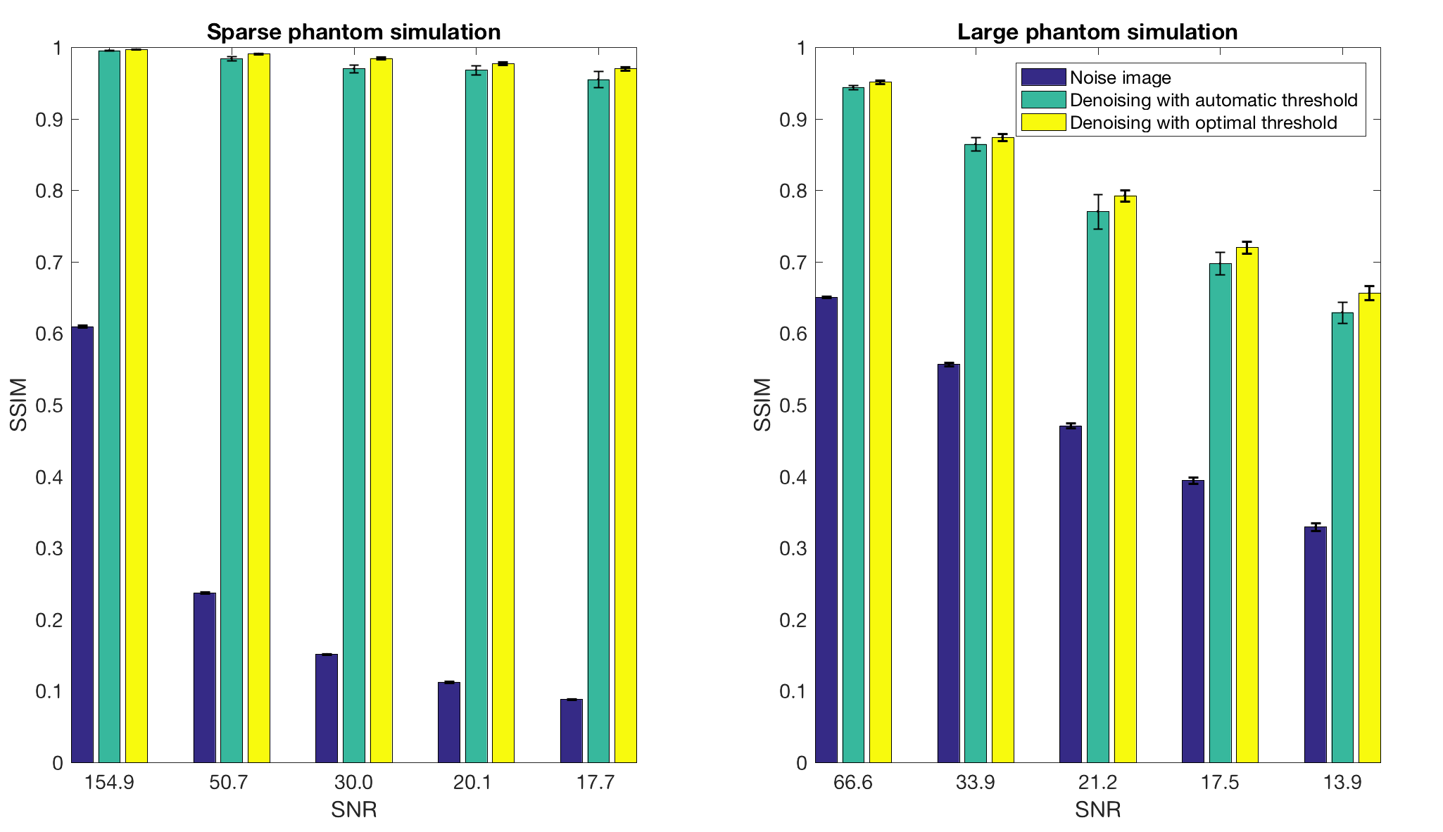
Simulations: The denoising method was demonstrated through simulations of a large and a sparse object. Five different levels of complex Gaussian noise were added to simulated multi-channel k-space datasets and 100 noise realizations were run to estimate SNR. To evaluate the quality of the automatically chosen threshold, the optimal threshold was found for each simulation based on the highest structural similarity (SSIM)5 to the true image.
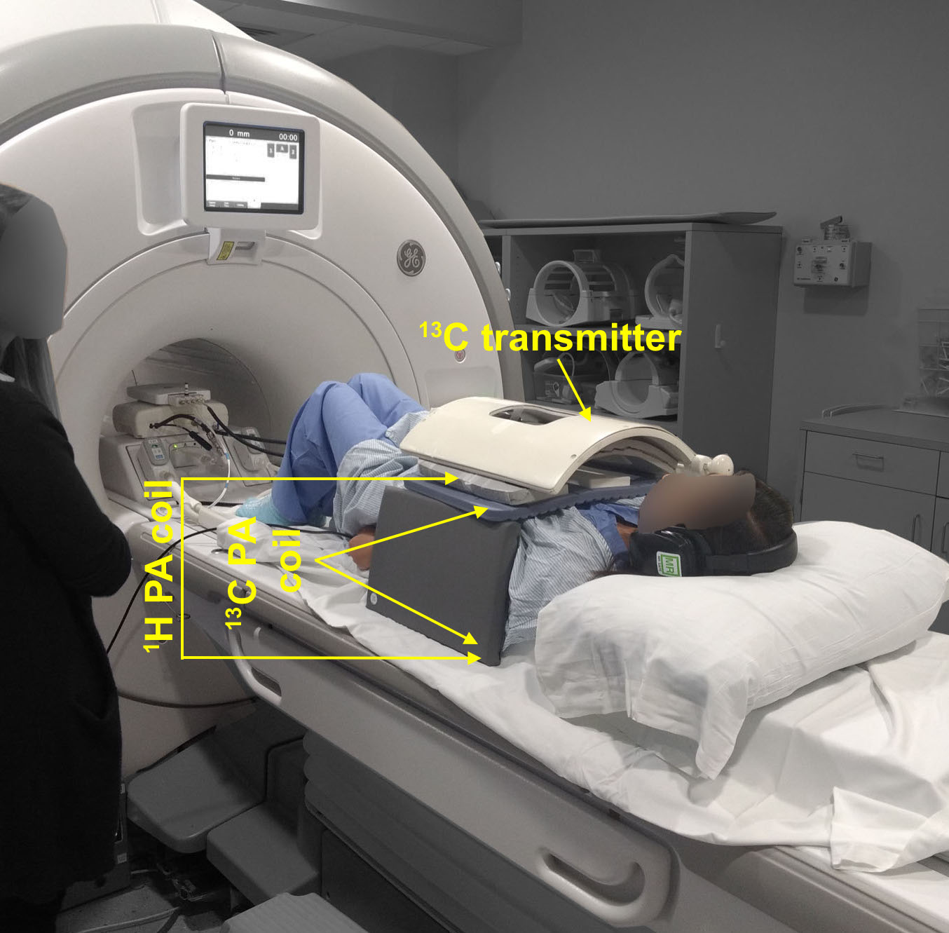
In vivo experiment: In vivo 13C data for a patient with metastases to the liver were acquired in a whole-body 3T MRI system (GE Healthcare, Waukesha, WI, USA) with a single-shot symmetric EPI readout after injection of hyperpolarized [1-13C]pyruvate.6 The multi-channel coil setup is shown in Figure 1. A singleband spectral-spatial RF pulse was used to selectively excite pyruvate, lactate, and alanine. Each metabolite volume consisting of 5 slices was acquired within 300 ms with a 2.1 s interval between time frames, yielding a 3-s temporal resolution. 20 total time frames were acquired. In-plane resolution (1.8x1.8 cm2), slice thickness (2 cm) and flip angles (38° pyruvate, 68° lactate/alanine) were chosen to match a concurrent single-slice spectroscopic imaging study (EPSI, not shown). After noise pre-whitening, automatic threshold reconstruction for denoising was performed. Kinetic modeling to estimate conversion rates of pyruvate to lactate (kPL), was performed both before and after denoising. Mean noise levels were subtracted to achieve zero mean. kPL was estimated by fitting the lactate signal at each time point, while pyruvate signal was taken as is, eliminating the need to make assumptions about the input function.7 Assumptions made: Fixed T1 of 25 s, unidirectional conversion and zero initial lactate signal.
Results and Discussion
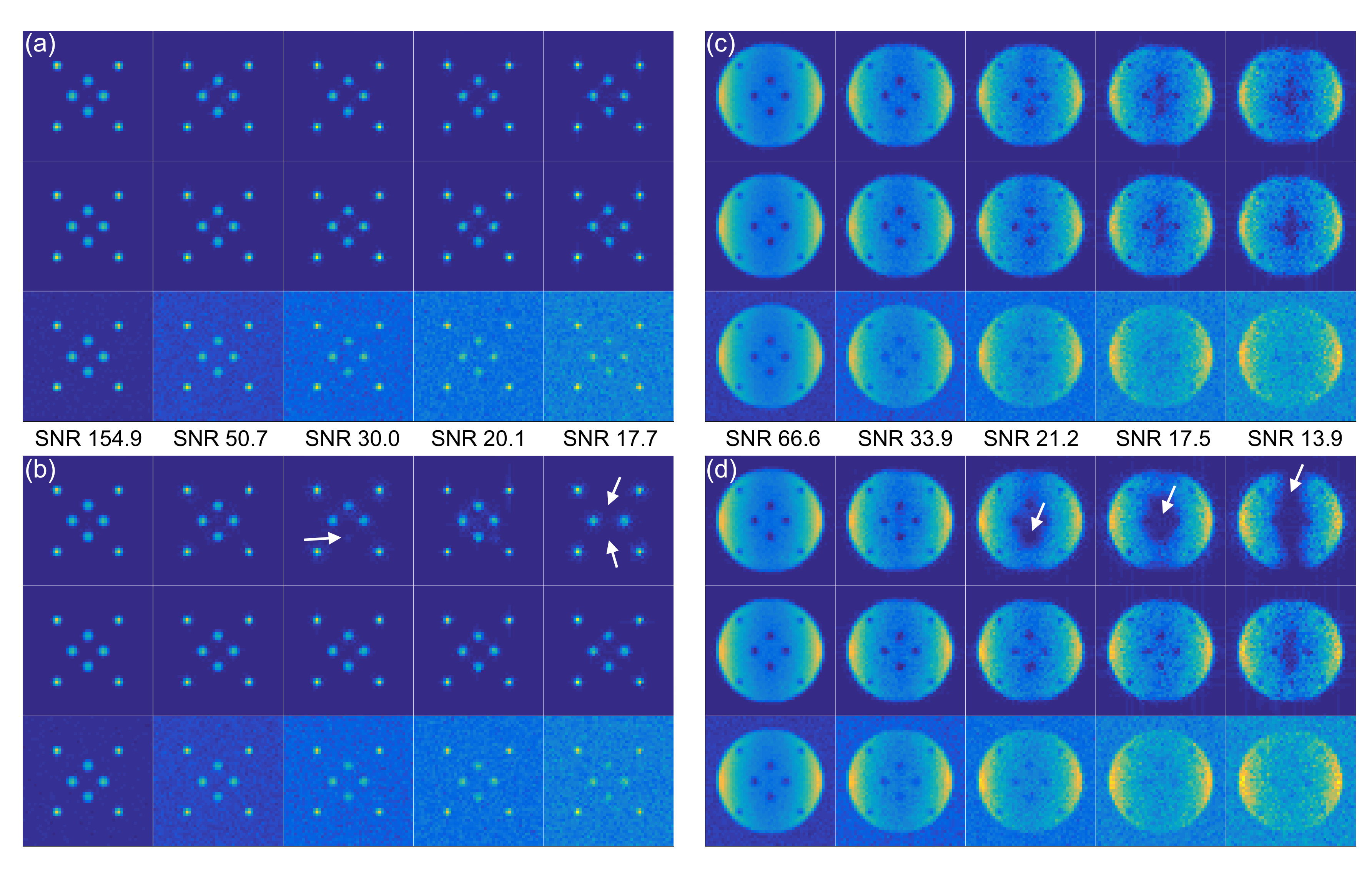
Figure 2 shows the best and worst-case simulation results. Figure 2(a) and (c) demonstrate the denoising method with a correctly chosen threshold, while (b) and (d) show the severity of artifacts when the threshold is underestimated. Figure 3 illustrates that automatic threshold reconstruction works similarly to optimal threshold reconstruction, which promotes its potential use in vivo when no gold standard exists. More robust threshold estimation is made for higher SNR levels.
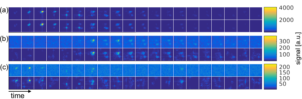
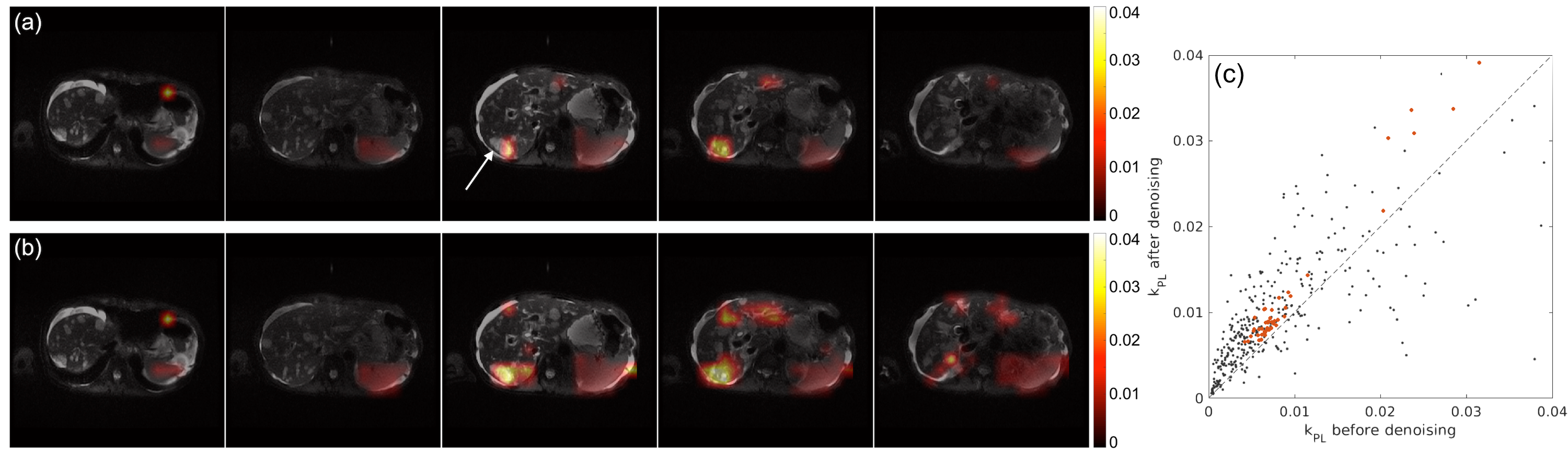
Figure 4 shows all time frames for the first slice from the in vivo dataset. The denoising effect is most evident for the lactate and alanine images. These images, however, also reveal suboptimal performance of the method for noise-only images. Figure 5 shows the kinetic modeling results. Only voxels where the fitting achieved r2 > 0.7 were overlaid on the proton images. This was a total of 119 voxels after denoising, compared to only 48 before. The arrow in (a) points to a liver metastasis region where a good fit was not attainable before denoising. The fitted kPL values with r2 > 0.7 in the scatter plot in (c) indicate a slight positive bias after denoising, which might be related to the fact that while the denoising method reduces background noise, additive noise is still contained in the signal subspace.
Conclusion
This study demonstrated advances in the analysis for multichannel human 13C liver imaging, resulting in better signal coverage together with higher quality kPL fits after denoising. Simulation results for the presented denoising method demonstrated a high increase in image quality, but also potential artifacts. Future studies should take advantage of more priors, such as smoothness for the dynamic dimension. This may reduce artifacts.Acknowledgements
This work has been partly funded by the Independent Research Fund Denmark (DFF – 4005-00531), the Danish National Research Foundation (DNRF124), and the Elite Research travel grant (6161-00043B).References
1. Zhu, Z. et al. Hyperpolarized 13C Dynamic Breath-held Molecular Imaging to Detect Targeted Therapy Response in Patients with Liver Metastases. in Proc. Intl. Soc. Mag. Reson. Med. 1115 (2017).
2. Shin, P. J. et al. Calibrationless parallel imaging reconstruction based on structured low-rank matrix completion. Magn. Reson. Med. 72, 959–70 (2014).
3. Feng, Y. et al. Development and testing of hyperpolarized 13C MR calibrationless parallel imaging. J. Magn. Reson. 262, 1–7 (2016).
4. Cadzow, J. A. Signal Enhancement - A Composite Property Mapping Algorithm. IEEE Trans. Acoust. 36, 49–62 (1988).
5. Wang, Z., Bovik, A. C., Sheikh, H. R. & Simoncelli, E. P. Image quality assessment: From error visibility to structural similarity. IEEE Trans. Image Process. 13, 600–612 (2004).
6. Gordon, J. W. et al. Human Hyperpolarized C-13 MRI Using a Novel Echo-Planar Imaging (EPI) Approach. in Proc. Intl. Soc. Mag. Reson. Med. 728 (2017).
7. Maidens, J., Gordon, J. W., Arcak, M. & Larson, P. E. Optimizing Flip Angles for Metabolic Rate Estimation in Hyperpolarized Carbon-13 MRI. IEEE Trans. Med. Imaging 35, 2403–2412 (2016).
Figures