3544
Accelerating Compressed Sensing in Cartesian Parallel Imaging Reconstructions using an Efficient and Effective Circulant Preconditioner1Circuits and Systems Group, Delft University of Technology, Delft, Netherlands, 2C.J. Gorter Center for High-Field MRI, Leiden University Medical Center, Leiden, Netherlands, 3Philips Research Hamburg, Hamburg, Germany
Synopsis
Reconstruction methods in parallel imaging and compressed sensing problems are generally very time consuming, especially for a large number of coil elements. In this work, the image is reconstructed using the Split Bregman algorithm (SB). We present an efficient and effective preconditioner that reduces the number of iterations in the linear least squares step of SB by almost a factor of 5 as alternative to extra variable splitting. The designed preconditioner works for Cartesian sampling schemes and for different coil configurations. It has negligible initialization time and leads to an overall speedup factor of 2.5.
Introduction
High undersampling factors can be achieved by using Parallel Imaging (PI) and Compressed Sensing (CS)1-6. We use the Split Bregman algorithm (SB) to reconstruct the image in which solving a linear least squares problem, usually solved iteratively, is the most time-consuming part7. In Cartesian sampling, however, this part can be solved directly by using extra variable splitting8,9. Alternatively, the number of iterations can be reduced by using preconditioners, although in literature they either have high initialization costs due to patient-specific coil sensitivities10, or evaluation of the preconditioner is expensive11-13. In this work, we propose an efficient and accurate Fast Fourier Transform (FFT)-based preconditioner for Cartesian PI-CS reconstructions that takes the coil sensitivities on a patient-specific basis into account and has negligible initialization time. Our imaging results show that the proposed preconditioner framework provides a good starting point for accelerating non-Cartesian reconstructions.Theory
For each SB iteration a linear least squares problem of the form $$$\text{A}\textbf{x}=\textbf{b}$$$ has to be solved, where $$$\textbf{x}$$$ is the true image, $$$\textbf{b}$$$ is the weighted undersampled k-space data, and
$$\text{A}=\mu\sum_{i=1}^{\text{N}_\text{c}}\left(\text{R}\text{F}\text{S}_i\right)^H\text{R}\text{F}\text{S}_i +\lambda\left(\text{D}_x^H\text{D}_x+\text{D}_y^H\text{D}_y\right)+\gamma\text{W}^H\text{W}\qquad(1)$$
is the system matrix that remains constant throughout the SB iterations. Here, the $$$\text{S}_i $$$ are diagonal matrices representing complex coil sensitivity maps for each of the $$$\text{N}_\text{c}$$$ channels. Furthermore, $$$\text{F}$$$ is the discrete two-dimensional Fourier transform matrix, and the undersampling pattern is specified by the binary diagonal sampling matrix $$$\text{R}$$$. The regularization parameters $$$\lambda$$$ and $$$\gamma$$$ in (1) are promoting sparsity via the total variation constraint (employing differentiation matrices $$$\text{D}_x$$$ and $$$\text{D}_x$$$) and the unitary wavelet transform $$$\text{W}$$$, respectively.
The second and third term in (1) are block circulant with circulant blocks (BCCB) matrices and are diagonalized by the Fourier matrix $$$\text{F}$$$. Writing
$$\text{A}=\text{F}^H\text{F}\text{A}\text{F}^H\text{F}=\text{F}^H\text{K}\text{F}$$
we have
$$\text{K}=\mu\underbrace{\sum_{i=1}^{\text{N}_\text{c}}\text{F} \text{S}_i^H\text{F}^H\text{R}^H\text{R}\text{F}\text{S}_i \text{F}^H}_{\text{K}_c} + \lambda \underbrace{ \vphantom{\sum_{i=1}^{\text{N}\text{c}}}\text{F} \left( \text{D}_x^H\text{D}_x + \text{D}_y^H\text{D}_y \right)\text{F}^H}_{\text{K}_d}+ \gamma \underbrace{\vphantom{\sum_{i=1}^{\text{N}\text{c}}}\text{I}}_{\text{K}_w}$$
where $$$\text{K}_d$$$ and $$$\text{K}_w$$$ are diagonal, but $$$\text{K}_c$$$ is not. Most of the
energy in $$$\text{K}_c$$$ is located
around its main diagonal, however. Hence, we approximate the matrix $$$\text{K}_c$$$ by its diagonal to arrive
at a BCCB approximation of $$$\text{A}$$$ as
preconditioner for solving the linear system. The required steps can be efficiently
performed using FFTs.
Methods
MR Data Acquisition: A Philips Ingenia 3T dual transmit MR system was used to acquire in vivo data. A 12-element posterior receiver array and 15-channel head coil were used for reception in spine and brain, respectively, whereas the body coil was used for RF transmission. T1-weighted images were acquired using a standard clinical TSE sequence and IR-TSE sequence for spine and brain, respectively.
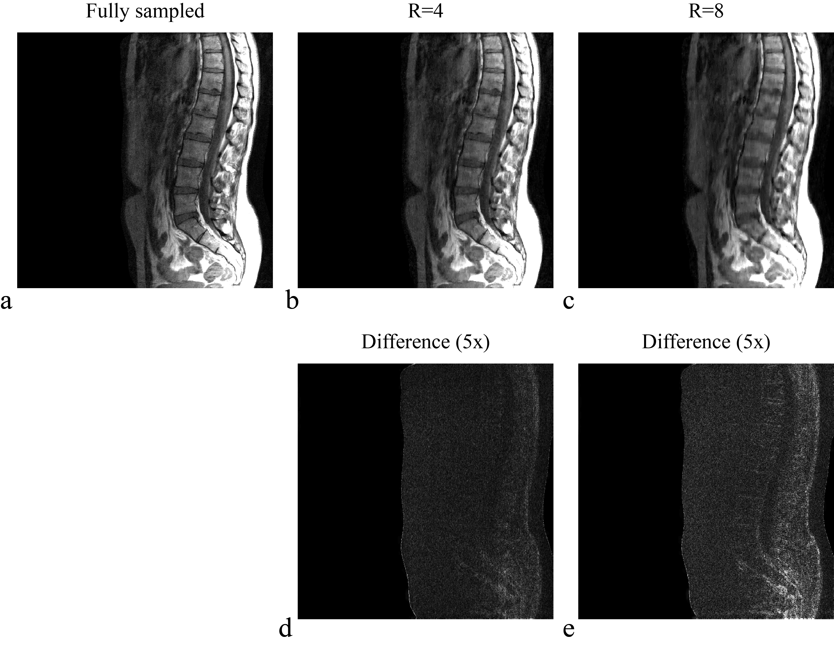
Reconstruction: The SB algorithm was implemented in MATLAB on a standard Windows 64-bit PC with 8 GB of internal memory. Unprocessed k-space data was stored per channel and used to construct cropped complex coil sensitivity maps14. Both the individual coil images and the coil sensitivity maps were normalized. Reconstruction for the spine data set was performed without and with coil compression15,16. A random line pattern and a fully random pattern, both with variable density, were studied for undersampling factors four (R=4) and eight (R=8).
Results
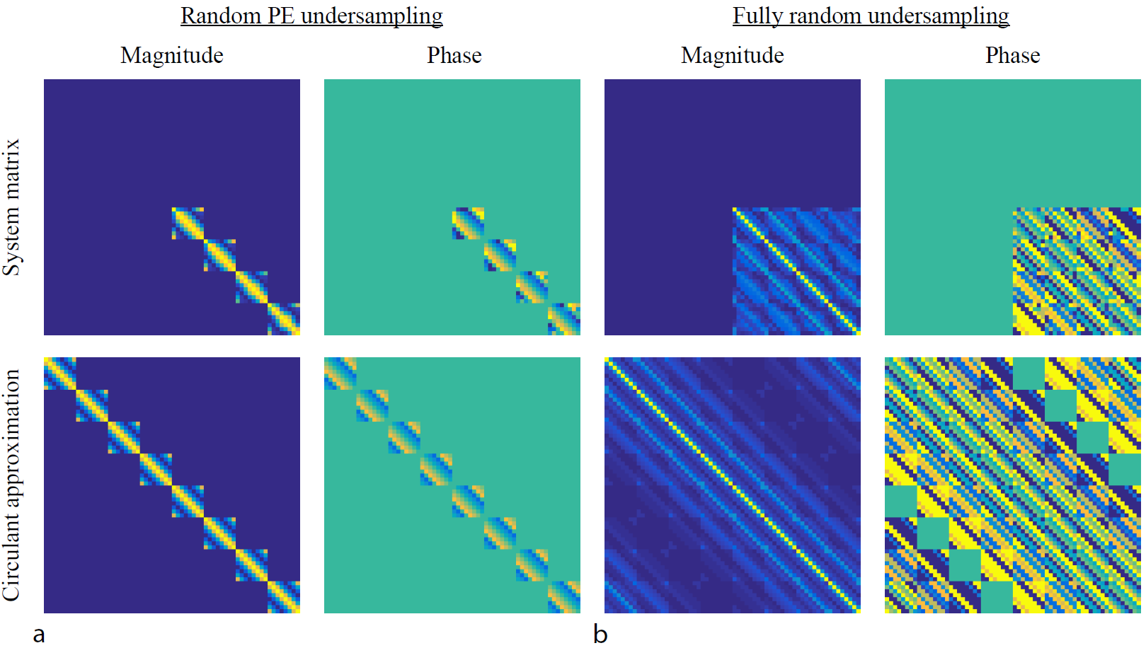
Figure 1 shows the TSE spine images for Cartesian undersampling factors R=4 and R=8. The full system matrix is constructed for illustration purposes only and compared with its circulant approximation in Fig. 2.
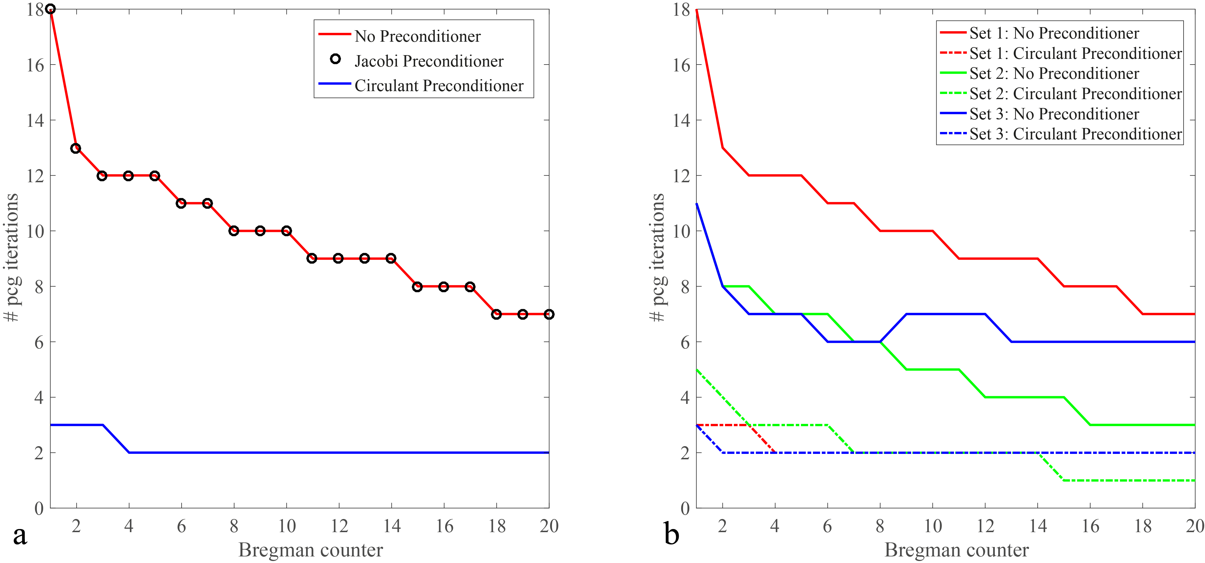
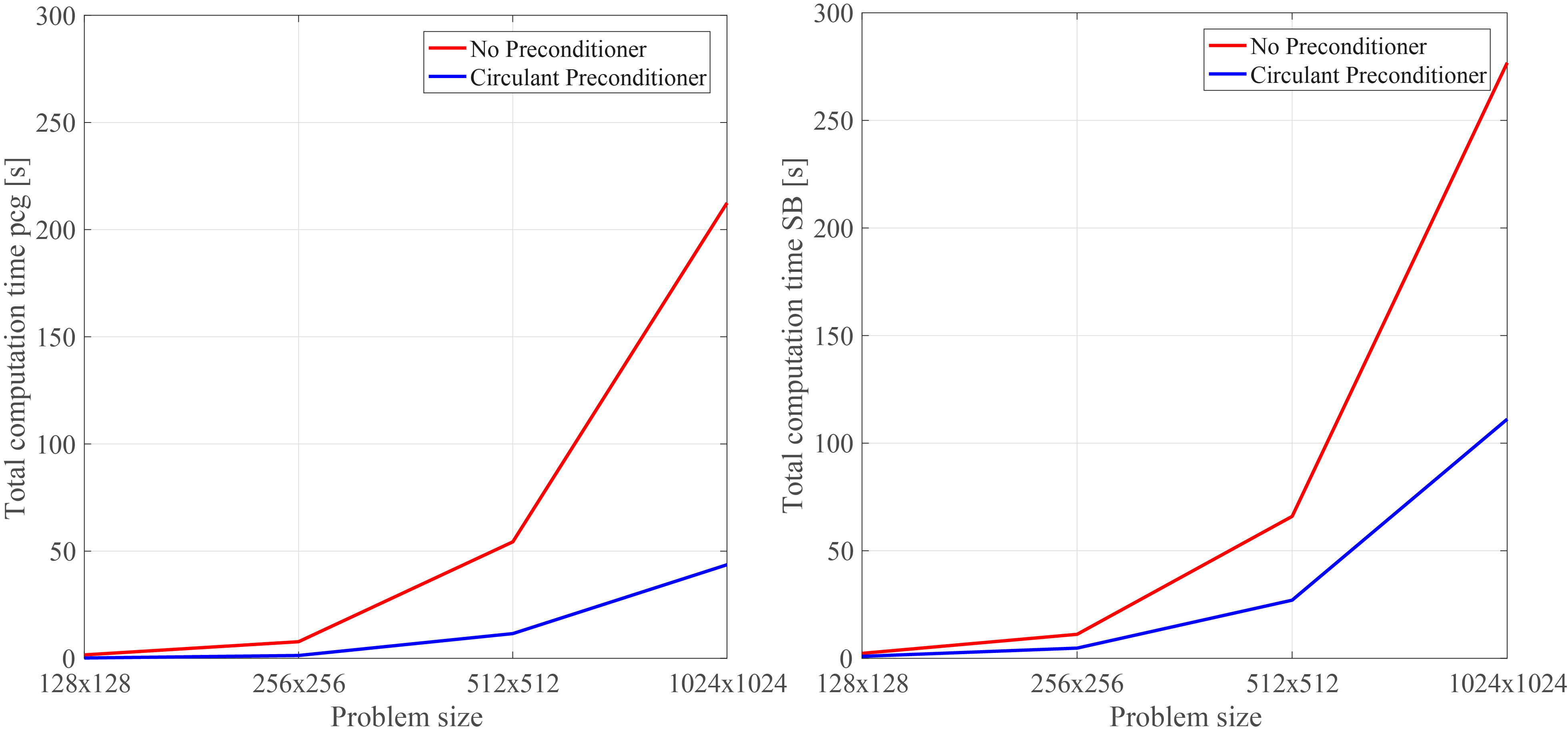
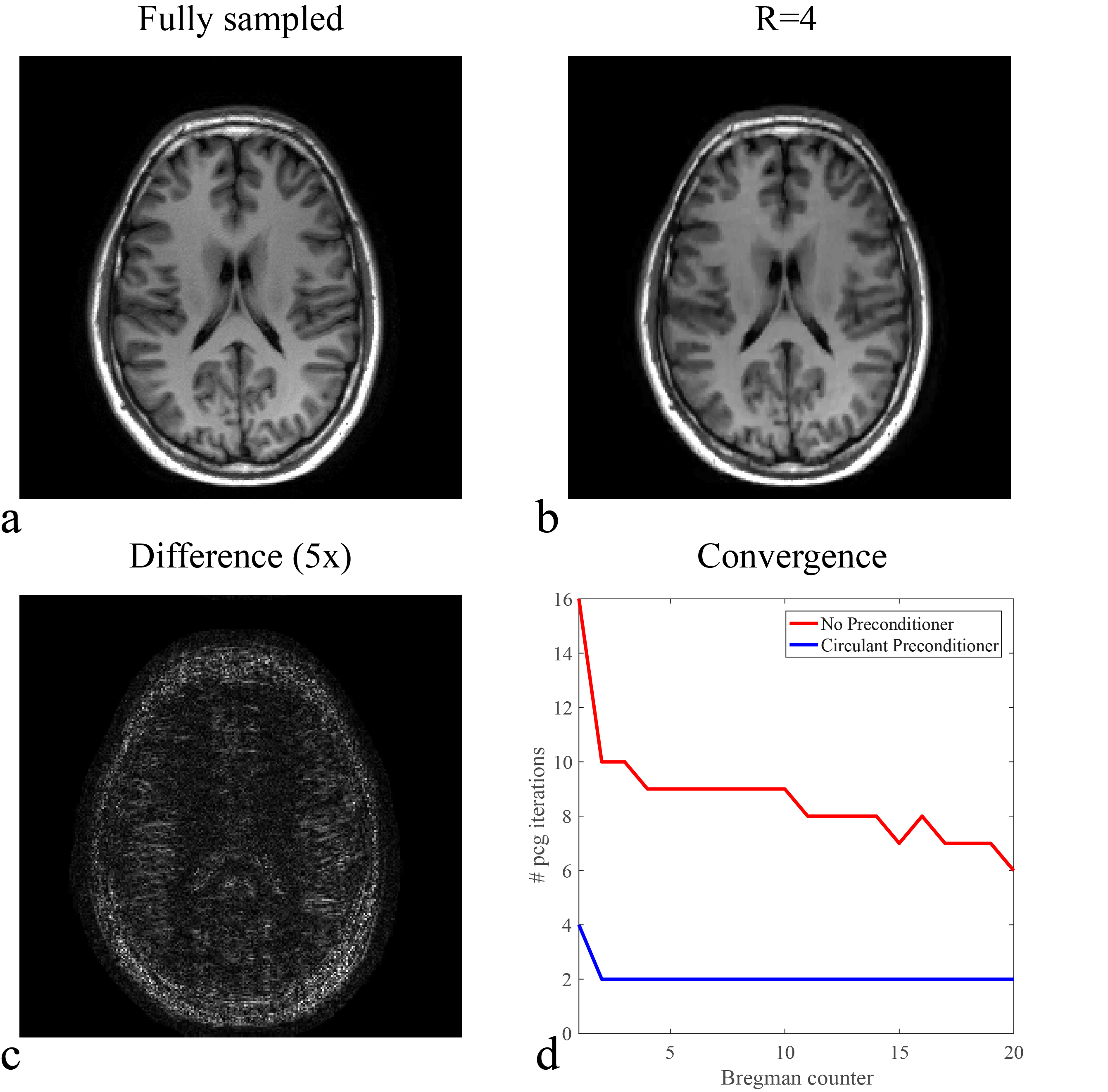
Figure 3a shows the number of iterations required for the preconditioned conjugate-gradient (PCG) solver to converge in each SB iteration without preconditioner, with the Jacobi preconditioner (the diagonal of matrix $$$\text{A}$$$), and with the circulant preconditioner proposed in this abstract. The reduced number of iterations leads to a shortened reconstruction time, plotted in Fig. 4a for the total PCG part in the SB algorithm (4.65x), and in Fig. 4b for the entire reconstruction algorithm (2.5x). For all matrix sizes the initialization time of the preconditioner is less than 2% of the image reconstruction time. Similar results are obtained for the 15-channel head coil as shown in Fig. 5.
Discussion and Conclusion
We have presented a circulant preconditioner that reduces the reconstruction times considerably for Cartesian CS-PI problems by solving the least-squares problem in the SB algorithm almost 5 times faster than without preconditioning, resulting in an overall reconstruction speedup factor of about 2.5. Without loss of performance it supports further speed up through coil compression, and works well for different coils and undersampling factors. The preconditioner has negligible initialization and evaluation time and is therefore highly scalable. In future work, our method will be compared in performance to extra variable splitting and extended to non-Cartesian sampling where direct solution methods are no longer feasible, possibly leading to faster reconstruction times.Acknowledgements
We would like to thank Ad Moerland from Philips Healthcare Best (The Netherlands) and Mariya Doneva from Philips Research Hamburg (Germany) for helpful discussions on reconstruction.
References
1. Pruessmann K et al. SENSE: Sensitivity Encoding for Fast MRI. Magnetic Resonance in Medicine, 1999; 42(5):952-962.
2. Griswold M et al. Generalized Autocalibrating Partially Parallel Acquisitions (GRAPPA). Magnetic Resonance in Medicine. 2002; 47(6):1202-1210.
3. Blaimer M et al. SMASH, SENSE, PILS, GRAPPA: How to Choose the Optimal Method. Topics in Magnetic Resonance Imaging. 2004; 15(4):223-236.
4. Deshmane A et al. Parallel MR imaging. Journal of Magnetic Resonance Imaging. 2012; 36(1):55-72
5. Donoho D et al. Compressed Sensing. IEEE Transactions on Information Theory. 2006; 52(4):1289-1306.
6. Lustig M et al. Sparse MRI: The Application of Compressed Sensing for Rapid MR Imaging. Magnetic Resonance in Medicine. 2007; 58(6):1182-1195
7. Goldstein T et al. The split Bregman Method for L1-Regularized Problems. SIAM Journal on Imaging Sciences. 2009; 2(2):323-343.
8. Ramani A et al. Parallel MR Image Reconstruction using Augmented Lagrangian Methods. IEEE Trans Med Imaging. 2011;30(3):694-706.
9. Weller D et al. Augmented Lagrangian with Variable Splitting for Faster Non-Cartesian L1-SPIRiT MR Image Reconstruction. IEEE Trans Med Imaging. 2014;33(2):351-361.
10. Saad Y. Iterative methods for sparse linear systems. Society for Industrial and Applied Mathematics. 2003; 2.
11. Chen C et al. Real Time Dynamic MRI with Dynamic Total Variation. International Conference on Medical Image Computing and Computer-Assisted Intervention. 2014;138-145
12. Li R et al. Fast Preconditioning for Accelerated Multi-contrast MRI Reconstruction. International Conference on Medical Image Computing and Computer-Assisted Intervention. 2015,700-707.
13. Xu Z et al. Efficient Preconditioning in Joint Total Variation Regularized Parallel MRI Reconstruction. International Conference on Medical Image Computing and Computer- Assisted Intervention. 2015;563-570.
14. Uecker M et al. ESPIRiT - An Eigenvalue Approach to Autocalibrating Parallel MRI: Where SENSE Meets GRAPPA. Magnetic Resonance in Medicine. 2014; 71(3):990-1001.
15. Huang F et al. A Software channel compression technique for faster reconstruction with many channels. Magnetic Resonance Imaging. 2008; 26(1):133-141.
16. Zhang T et al. Coil Compression for Accelerated Imaging with Cartesian Sampling. Magnetic Resonance in Medicine. 2013; 69(2):571-582.
Figures