Synopsis

We present our updated results in the evaluation of the Normalised Iterative Hard Thresholding Algorithm (NIHT) for parallel imaging and compressed sensing reconstructions of highly accelerated Cardiac cine MRI at 7 Tesla. We compare imaging performance with three other parallel imaging and compressed sensing methods, including regularisation in the temporal dimension.

INTRODUCTION

METHODS

Sparse signal recovery can be posed as the following optimisation problem:

$$x^*=\underset{x\,:\,\|x\|_0\leq K}{\operatorname{arg\,min}}{\|y-\Phi x\|}_2$$

where $$$y$$$ represents the k-space measurements, $$$x$$$ is the image or its sparse representation, and $$$\Phi$$$ is the linear mapping operator that maps $$$x$$$ to $$$y$$$. Assuming that the image vector, or its representation, is sparse, we are looking for a vector $$$x^*$$$ which minimises the error $$${\| y - \Phi x \|}_2$$$ with the constraint that $$$x$$$ has at most $$$K$$$ non-zero elements. The number of non-zeros in a vector is indicated by the operator $$${\| \cdot \|}_0$$$.

The NIHT algorithm performs reconstruction using gradient descent iterations each followed by the thresholding step:

$$x^{n+1}= H_K \left(x^n +\mu^n \Phi^T \left( y - \Phi x^n \right)\right)$$

where $$$H_K$$$ is the non-linear operator that keeps the $$$K$$$ largest magnitude elements of a vector and sets the rest to zero, and $$$\mu^n$$$ is an adaptive step size to maximally reduce the error at each iteration. We chose to use a representation of $$$x$$$ in the wavelet domain. We also consider thresholding to the $$$K$$$ largest elements consistent across the time dimension, which we refer to as joint thresholding.

We examined the performance of NIHT, along with three other methods: $$$l_2$$$ regularisation with conjugate gradients, Iterative Soft Thresholding (IST)⁴ using wavelets, including joint thresholding in the time dimension, and Total Variation (TV)⁵ in the time dimension. All algorithms are applied with parallel imaging using SENSE,⁶ where the sensitivities are estimated from the fully sampled k-space with the ESPIRiT⁷ method.

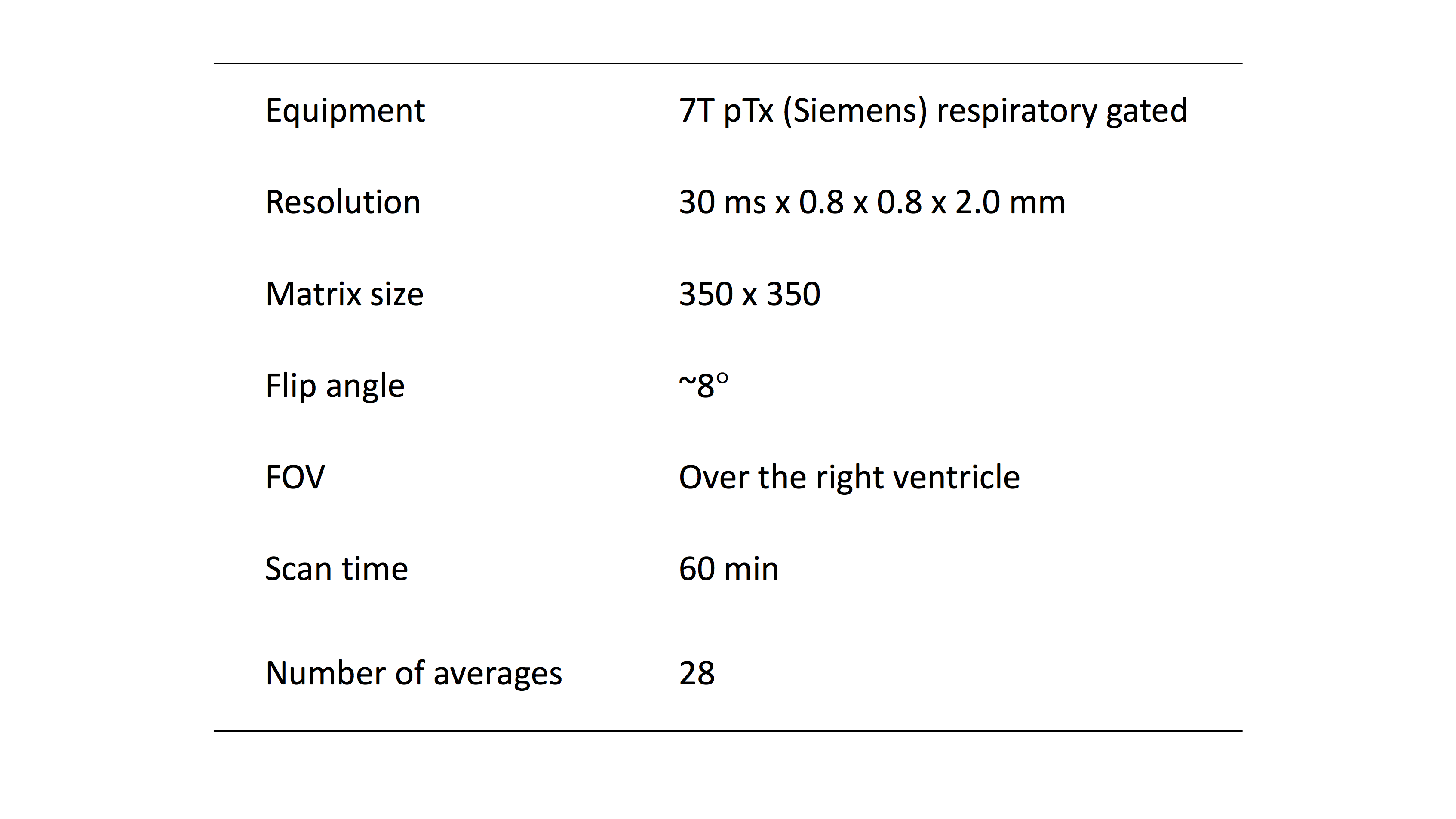
We performed tests on data acquired from a single healthy subject. A Fully sampled, free breathing 2D GRE cine, was synthetically undersampled in 2D, so as to emulate undersampling in the two phase-encoding directions of a 3D Cartesian acquisition. The relevant cine MRI parameters⁸ are listed in the table of figure 1.

We applied 2D variable density Poisson disk sampling masks⁹ on the data to produce acceleration rates between 2.09 to 46.44. Images were then reconstructed with each method, and compared to the fully sampled SENSE reconstruction over a region of interest, containing mainly the heart. We calculated the Root Mean Squared Error (RMSE), and the Structural Similarity Index (SSIM),¹⁰ the latter being generally considered to provide a better measure of perceptual visual fidelity. The algorithms were also run with a range of regularisation parameters for each method, and the ones yielding the lowest RMS and highest SSIM were chosen.

RESULTS

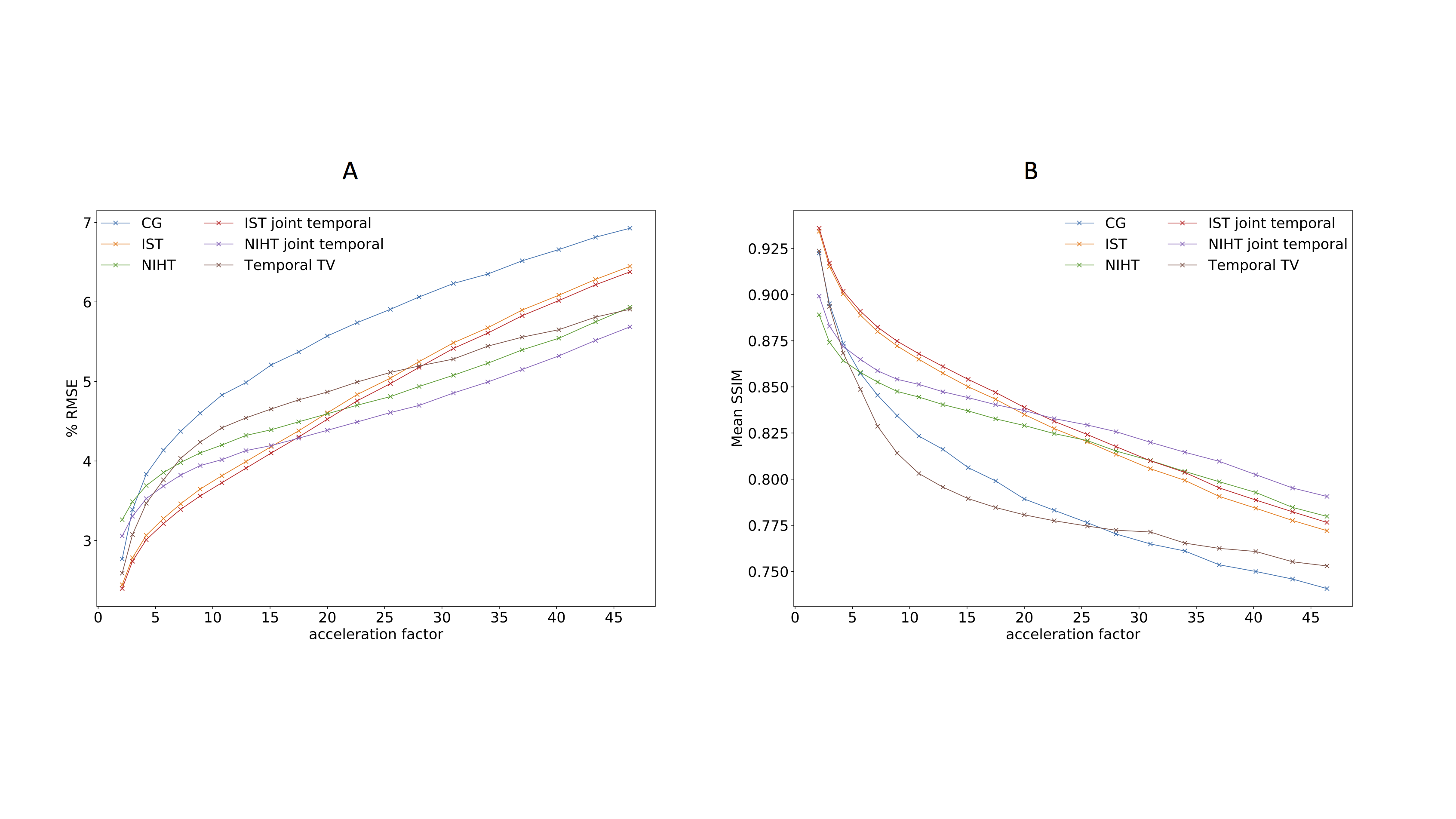
The RMSE and SSIM are plotted in figure 2. Better RMSE performance is observed for the joint NIHT for accelerations above ~17.5, with a lower rate of RMSE increase across acceleration for both NIHT and joint NIHT, compared to IST. For accelerations lower than ~15, IST achieves the best RMSE. In terms of SSIM, the joint NIHT appears superior above an acceleration of ~20.

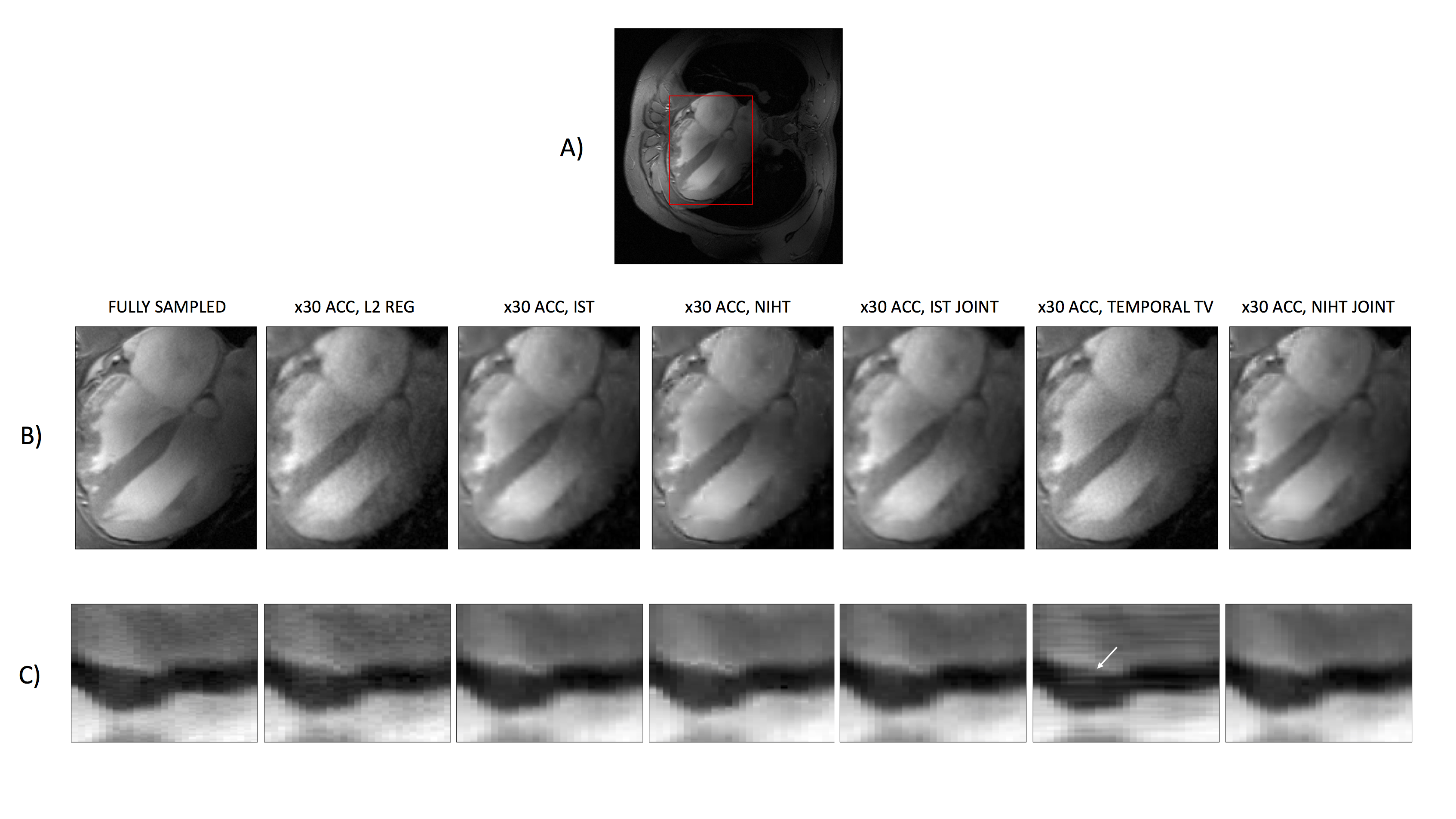
Figure 3 shows accelerations of 30-fold, along with a spatial-temporal profile for a line crossing the septum. We do not observe any significant advantage between the algorithms in their spatial-temporal profile, however TV appears to have increased temporal blurring in a region of boundary change.

DISCUSSION

CONCLUSIONS

Acknowledgements

References

1. Blumensath, T., & Davies, M. E. (2010). Normalized iterative hard thresholding: Guaranteed stability and performance. IEEE Journal of selected topics in signal processing, 4(2), 298-309. doi:10.1109/JSTSP.2010.2042411
2. Tamir, J I., Ong, F., Cheng, J. Y., Uecker, M., and Lustig, M., (2016), Generalized Magnetic Resonance Image Reconstruction using The Berkeley Advanced Reconstruction Toolbox, ISMRM Workshop on Data Sampling and Image Reconstruction, Sedona 2016
3. BART (https://mrirecon.github.io/bart/) (2017) DOI: 10.5281/zenodo.817472
4. Daubechies, I., Defrise, M. and De Mol, C. (2004), An iterative thresholding algorithm for linear inverse problems with a sparsity constraint. Comm. Pure Appl. Math., 57: 1413–1457. doi:10.1002/cpa.20042
5. Feng, L., Srichai, M. B., Lim, R. P., Harrison, A., King, W., Adluru, G., Dibella, E. V. R., Sodickson, D. K., Otazo, R. and Kim, D. (2013), Highly accelerated real-time cardiac cine MRI using k–t SPARSE-SENSE. Magn Reson Med, 70: 64–74. doi:10.1002/mrm.24440
6. Pruessmann KP, Weiger M, Scheidegger MB, Boesiger P. SENSE: sensitivity encoding for fast MRI. Magn Reson Med 1999; 42: 952–962.
7. Uecker, M., Lai, P., Murphy, M. J., Virtue, P., Elad, M., Pauly, J. M., Vasanawala, S. S. and Lustig, M. (2014), ESPIRiT—an eigenvalue approach to autocalibrating parallel MRI: Where SENSE meets GRAPPA. Magn. Reson. Med., 71: 990–1001. doi:10.1002/mrm.24751
8. Hess, A. T., Tunnicliffe, E. M., Rodgers, C. T. and Robson, M. D. (2017), Diaphragm position can be accurately estimated from the scattering of a parallel transmit RF coil at 7 T. Magn. Reson. Med. doi:10.1002/mrm.26866
9. Lustig, M., Donoho, D. and Pauly, J. M. (2007), Sparse MRI: The application of compressed sensing for rapid MR imaging. Magn. Reson. Med., 58: 1182–1195. doi:10.1002/mrm.21391
10. Wang, Z., Bovik, A. C., Sheikh, H. R., & Simoncelli, E. P. (2004). Image quality assessment: from error visibility to structural similarity. IEEE transactions on image processing, 13(4), 600-612. doi:10.1109/TIP.2003.819861