3532
Gini reweighted ℓ1 minimization for rapid MRI1Department of Electrical Engineering, Pontificia Universidad Católica de Chile, Santiago, Chile, 2Biomedical Imaging Center, Pontificia Universidad Católica de Chile, Santiago, Chile, 3Division of Imaging Sciences and Biomedical Engineering, King’s College London, London, United Kingdom, 4Institute for Computational and Mathematical Engineering, Stanford University, Stanford, CA, United States, 5Institute for Biological and Medical Engineering, Pontificia Universidad Católica de Chile, Santiago, Chile
Synopsis
Under-sampling acquisition is oftenly used to reduce the scan time. Compressed Sensing allows the reconstruction of these data by solving a convex optimization problem. This is done to exploit the sparsity of the signals using the ℓ1-norm. We propose to use the Gini Index as a sparsity measure. In this work we demonstrate that this index allow to further increase the under-sampling factor. Interestingly this non-linear index can be computed by solving iteratively reweighted ℓ1 problems, without excessive computational load.
Introduction
Faster imaging is achieved by under-sampling the acquisition in $$$k$$$-space. Images can be recovered assuming sparsity by a Compressed Sensing1,2 reconstruction which can be expressed as3,4$$ \min_{\vec{x}\in\mathbb{C}^{N}}\quad\,\left\Vert \vec{x}\right\Vert _{1}\quad\quad\quad[1]\\s.t.\quad\left\Vert \Phi\Psi\vec{x}-\vec{y}\right\Vert _{2}\leq\epsilon,$$with $$$ \Psi\in\mathbb{C}^{N\times N}$$$ the basis of a dictionary, $$$ \Phi\in\mathbb{C}^{M\times N}$$$ the matrix to represent the measure domain and $$$ \vec{y}\in\mathbb{C}^{M}$$$ the acquired data. Using the ℓ1-norm is a practical way to measure sparsity, we propose to use another that satisfies desirable properties to measure sparsity5 and also is affordable computationally. The Gini Index (GI)6,7 is a measure that has all the desirable properties5. Furthermore, a simple formulation can be achieved if a sorting operation is performed beforehand. Thus, if $$$ \left|x_{\left[1\right]}\right|\leq\left|x_{\left[2\right]}\right|\leq\dots\leq\left|x_{\left[N\right]}\right|$$$ then we can represent the GI as a weighted ℓ18$$\mathrm{GI}\left(\vec{x}\right) =1-2\sum_{n=1}^{N}\underbrace{\left(\frac{N-n+\frac{1}{2}}{N}\right)}_{w_{n}}\frac{\left|x_{\left[n\right]}\right|}{\left\Vert \vec{x}\right\Vert _{1}}\\ =1-2\left\Vert \frac{\vec{w}^{\mathrm{T}}}{\left\Vert \vec{x}\right\Vert _{1}}\cdot\left(\mathcal{P}\vec{x}\right)\right\Vert _{1}\\ =1-2\left\Vert \vec{W}_{\vec{x}}^{\mathrm{T}}\cdot\vec{x}\right\Vert _{1}\quad\,\,[2],$$Where $$$ \mathcal{P}$$$ is a permutation matrix that represent the sorting unitary operator and $$$ \vec{W}_{\vec{x}}=\mathcal{P}^{\mathrm{T}}\vec{w}/\left\Vert \vec{x}\right\Vert _{1}$$$. Because of this, the use in inverse problems has been explored by replacing the ℓ1-norm by the weighted ℓ19.
Methods
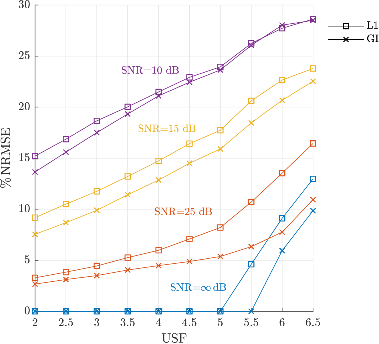
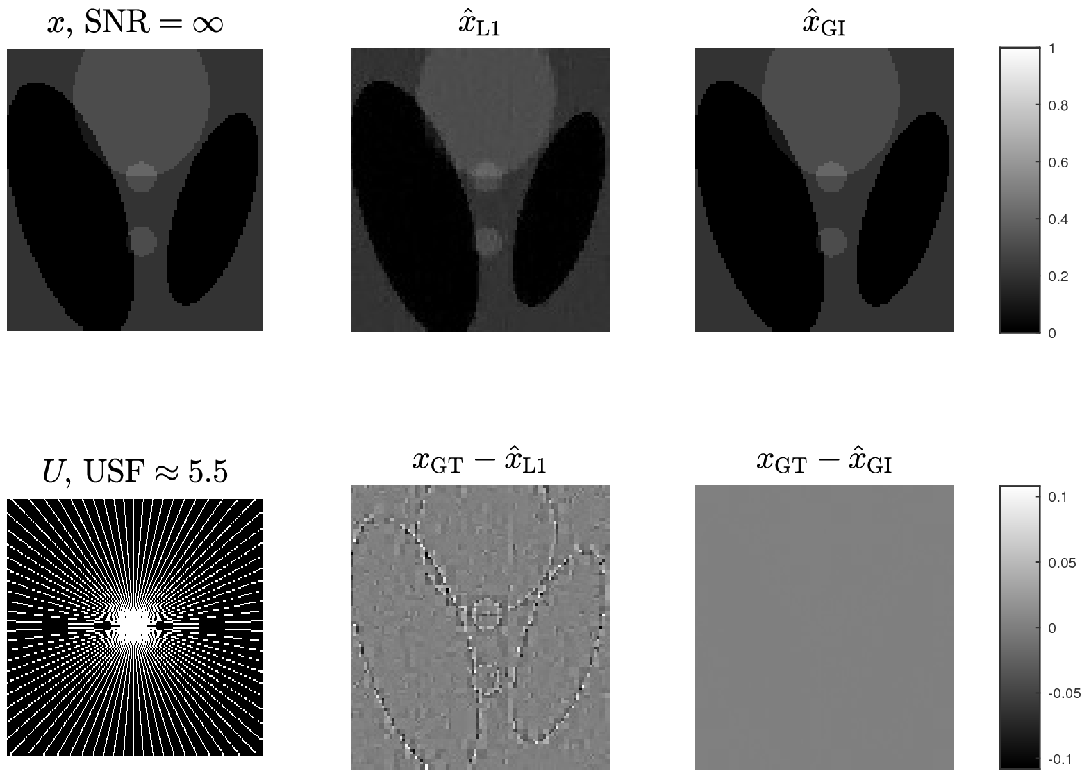
One of the problems of solving [1] with [2] is that the function is not convex and uses a sorting operation. In order to solve this problem we implemented an iteratively reweighted ℓ1 algorithm10,11,12 as pointed in [3].$$\vec{x}^{k+1}=\underset{x\in\mathcal{C}_{\epsilon}}{\mathrm{argmin}}\,\left\Vert \vec{W}_{\vec{x}^{k}}^{\mathrm{T}}\cdot\vec{x}\right\Vert _{1},\quad\mathcal{C}_{\epsilon}=\left\{ \vec{x}:\left\Vert \Phi\Psi\vec{x}-\vec{y}\right\Vert _{2}\leq\epsilon\right\} .\quad [3]$$The updates of the weight vector are done as previously described. To solve each optimization problem we used the SPGL1 solver13,14.A numerical phantom was tested for various Under-Sampling Factors (USF) and Signal-to-Noise Ratios (SNRs) by adding complex gaussian noise. Additionally, we tested the GI with one real data set (brain image). Each experiment used a Haar and Daubechies (db4) with level of decomposition 4 wavelet as the sparsifying transform. The measurement operator was an under-sampled Fourier transform that uses radial $$$k$$$-space trajectory for the phantom and polynomial variable density under-sampling for the brain. The maximum amount of iterations in [3] was $$$k^{\mathrm{phantom}}_{\max}=5$$$ and $$$k^{\mathrm{brain}}_{\max}=10$$$, and a stopping criterion as described in previous works9 was used. The results were compared with the Normalized Root Mean Squared Error (NRMSE), which is defined as follows$$\mathrm{NRMSE}\{x,x0\}=\frac{\Vert x-x_0\Vert_2}{\Vert x_0 \Vert_2}.$$Results and discussion
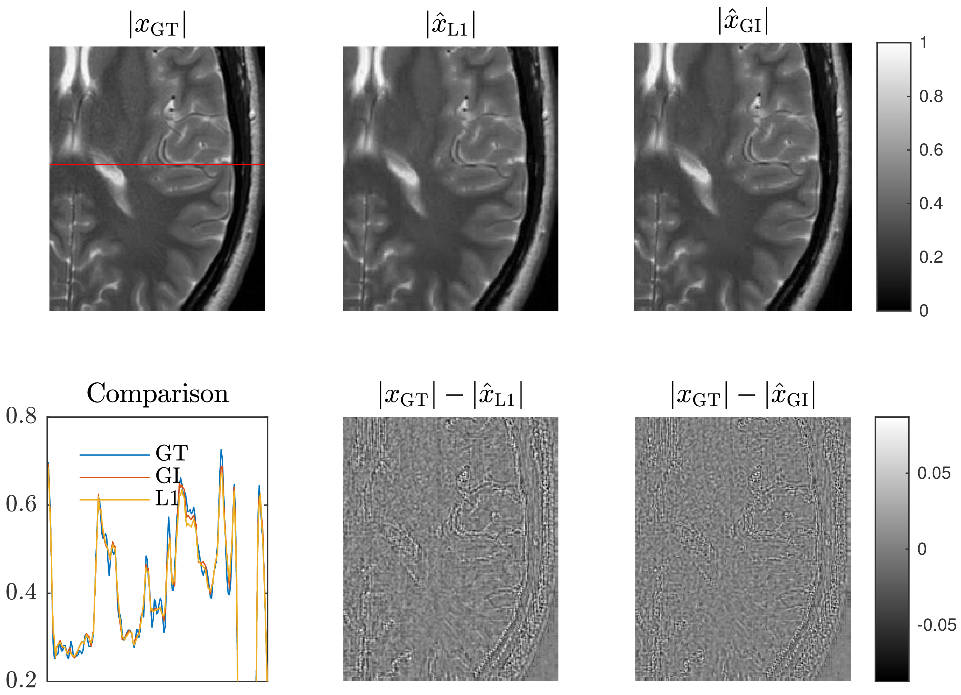
As seen in Figure 1 the GI sparsity measure performs considerably better compared to ℓ1 for SNR greater than 15 dB, and comparable for SNR of 10 dB. In Figure 2 we can see that for a simple digital phantom a perfect reconstruction is achieved for larger USF using the GI. An improvement for the brain image quality, Figure 3, can also be observed, although the results are less significant than for the phantom, due to the noise level.Conclusion
The GI is a good sparsity measure that satisfies many desirable properties5. The proposed method performed well in the numerical phantom with less or equal NMRSE than the ℓ1-norm even achieving perfect reconstruction at higher USFs, replicating already existing studies7,9. The in-vivo results are also better, although not significant for the particular case we tested. In summary, the GI improves the reconstruction for under-sampled acquisitions and we believe it must be further explored for MRI reconstruction or other ℓ1-based problems.
Acknowledgements
The authors gratefully acknowledge CONICYT for funding this research through PIA-Anillo ACT1416.References
1. Lustig M, Donoho D, Pauly JM. Sparse MRI: The application of compressed sensing for rapid MR imaging. Magnetic Resonance in Medicine 2007; 58:1182–1195.
2. Candès EJ, Wakin MB. An Introduction To Compressive Sampling. IEEE Signal Processing Magazine 2008;25:21–30.
3. Candès EJ, Romberg J, Tao T. Robust uncertainty principles: exact signal reconstruction from highly incomplete frequency information. IEEE Transactions on Information Theory 2006; 52:489–509.
4. Candès EJ, Romberg JK, Tao T. Stable signal recovery from incomplete and inaccurate measurements. Communications on Pure and Applied Mathematics 2006;59:1207–1223.
5. Hurley N, Rickard S. Comparing Measures of Sparsity. IEEE Transactions on Information Theory 2009;55:4723–4741.
6. Damgaard C, Weiner J. Describing Inequality in Plant Size or Fecundity. Ecology 2000; 81:1139–1142.
7. Zonoobi D, Kassim AA, Venkatesh YV. Gini Index as Sparsity Measure for Signal Reconstruction from Compressive Samples. IEEE Journal of Selected Topics in Signal Processing 2011; 5:927–932.
8. Huang XL, Shi L, Yan M. Nonconvex sorted ℓ1 minimization for sparse approximation. Journal of the Operations Research Society of China 2015; 3:207–229.
9. Feng C, Xiao L, Wei ZH. Compressive Sensing Inverse Synthetic Aperture Radar Imaging Based on Gini Index Regularization. International Journal of Automation and Computing 2014; 11:441–448.
10. Ochs P, Dosovitskiy A, Brox T, Pock T. On iteratively reweighted algorithms for nonsmooth nonconvex optimization in computer vision. SIAM Journal on Imaging Sciences 2015; 8:331–372.
11. Candès EJ, Wakin MB, Boyd SP. Enhancing Sparsity by Reweighted l1 Minimization. Journal of Fourier Analysis and Applications 2008; 14:877–905.
12. Bogdan M, van den Berg E, Sabatti C, Su W, Candès EJ. Slope adaptive variable selection via convex optimization. The annals of applied statistics 2015; 9:1103–1140.
13. van den Berg E, Friedlander MP. SPGL1: A solver for large-scale sparse reconstruction, June 2007,http://www.cs.ubc.ca/labs/scl/spgl1.
14. van den Berg E, Friedlander M. Probing the Pareto Frontier for Basis Pursuit Solutions. SIAM Journal on Scientific Computing 2008; 31:890–912.
Figures